Next: 5.2 Integrating the path
Up: 5. Computing the kernel
Previous: 5. Computing the kernel
5.1 Integrating the functional wave equation
It is possible to compute
K [ x (s) , x 0 (s) ; A] exactly
in the ``free'' case because the
Lagrangian corresponding to the Hamiltonian (2) is
quadratic with respect to the generalized velocities
 .
Previous experience with this class of Lagrangians
suggests the following ansatz for the string quantum kernel:
.
Previous experience with this class of Lagrangians
suggests the following ansatz for the string quantum kernel:
![\begin{displaymath}K _{0} [ x (s) , x _{0} (s) ; A]
=
\mathcal{N}
A ^{\alpha}...
...\left(
i I [ x (s) , x _{0} (s) ; A ]
/
\hbar
\right)
\ ,
\end{displaymath}](img87.gif) |
(31) |
where
 is a normalization constant, and
  a real number.
Substituting this ansatz into eq.(29) gives two
independent equations for the amplitude and the phase
respectively,
a real number.
Substituting this ansatz into eq.(29) gives two
independent equations for the amplitude and the phase
respectively,
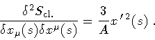
Comparing equations (33) and (11), we see that
![$I = S _{\mathrm{cl.}}[ x (s) , \, x _{0} (s) ; A]$](img94.gif) and (33) is just the classical Jacobi equation.
Therefore, the main problem is to determine the form of
S cl. in the string case. We do so by analogy with the
relativistic point-particle case, where
S cl. is a
functional of the world-line length element. Accordingly, we first
introduce the oriented
surface element as a functional of the surface boundary C
and (33) is just the classical Jacobi equation.
Therefore, the main problem is to determine the form of
S cl. in the string case. We do so by analogy with the
relativistic point-particle case, where
S cl. is a
functional of the world-line length element. Accordingly, we first
introduce the oriented
surface element as a functional of the surface boundary C
![\begin{displaymath}\sigma ^{\mu \nu} [ C ]
\equiv
\oint _{C} x ^{\mu} d x ^{\n...
...int _{0} ^{1} d u \, x ^{\mu} (u)
\frac{d x ^{\nu}}{d u}
\ .
\end{displaymath}](img95.gif) |
(34) |
Then, from the above definition we obtain
Next, we introduce the trial solution
| S cl.[ x (s) , x 0 (s) ; A] |
= |
![$\displaystyle \frac{\beta}{4 A}
\left(
\sigma ^{\mu \nu} [C]
-
\sigma ^{\mu \nu...
...]
\right)
\left(
\sigma _{\mu \nu} [C]
-
\sigma _{\mu \nu} [C _{0}]
\right)
\ ,$](img100.gif) |
|
| |
 |
![$\displaystyle \frac{\beta}{4 A}
\Sigma ^{\mu \nu} [ C - C _{0}]
\Sigma _{\mu \nu} [ C - C _{0}]$](img101.gif) |
(37) |
where  is a second parameter to be fixed by the equations
(32), (33). By taking into account (35),
(36), we find
is a second parameter to be fixed by the equations
(32), (33). By taking into account (35),
(36), we find
![\begin{displaymath}\frac{\delta S _{\mathrm{cl.}}}{\delta x ^{\mu} (s)}
=
\fra...
... \Sigma _{\mu \nu} [ C - C _{0} ]
x ^{\prime \, \nu} (s)
\ .
\end{displaymath}](img103.gif) |
(38) |
Note that the dependence on the parameter s is only through the
factor
 .
Then,
.
Then,
 |
(39) |
Equations (33) and (32) now give
 |
(40) |
Finally, if we define the loop space Dirac delta function
![\begin{displaymath}\delta [ C - C _{0} ]
\equiv
\lim _{\epsilon \rightarrow 0}...
...\nu} [ C - C _{0} ]
\Sigma _{\mu \nu} [ C - C _{0} ]
\right)
\end{displaymath}](img107.gif) |
(41) |
then, the kernel normalization constant is fixed by the boundary
condition (16), and we finally obtain the promised
expression of the quantum kernel as an exact evaluation of the path
integral
![\begin{displaymath}K [ x (s) , x _{0} (s) ; A ]
=
\left(
\frac{m ^{2}}{2 i \p...
...[ C - C _{0} ]
\Sigma _{\mu \nu} [ C - C _{0} ]
\right)
\ .
\end{displaymath}](img108.gif) |
(42) |
The above equation, in turn, leads us to the following
representation of the Nambu-Goto closed string propagator
| |
|
![$\displaystyle \int _{x _{0} (s)} ^{x(s)} [D x ^{\mu} (\sigma)]
\exp
\left\{
-
\...
...} \sigma
\sqrt{-\frac{1}{2}
{\dot{x}}^{\mu \nu}
{\dot{x}}_{\mu \nu}}
\right\}
=$](img109.gif) |
|
| |
|
![$\displaystyle \qquad =
\int _{0} ^{\infty} \! \! \! \! \! \! d A \,
e ^{- i m ^...
... A}
\Sigma ^{\mu \nu} [ C - C _{0} ]
\Sigma _{\mu \nu} [ C - C _{0} ]
\right)
.$](img110.gif) |
(43) |
Note that, since no approximation was used to obtain equation
(43), the above representation can also be interpreted as a
new definition of the
Nambu-Goto path integral. This definition is based on the classical
Jacobi formulation of string dynamics rather than on the customary
discretization procedure.
Next: 5.2 Integrating the path
Up: 5. Computing the kernel
Previous: 5. Computing the kernel
Stefano Ansoldi
Department of Theoretical Physics
University of Trieste
TRIESTE - ITALY


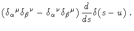
![$\displaystyle \frac{\delta \sigma ^{\mu \nu} [C]}{ \delta x ^{\alpha} (s)}$](img96.gif)
![$\displaystyle \frac{\delta ^{2} \sigma ^{\mu \nu} [C]}
{\delta x ^{\alpha} (s) \delta x ^{\beta} (u)}$](img98.gif)