Next: 3. Feynman and Jacobi
Up: String Propagator: a Loop
Previous: 1. Introduction
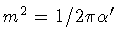
2. Functional Jacobi equation
As a starting point for the study of string dynamics one can
choose either the Nambu-Goto action, or the Schild action: both
functionals
lead to the same classical dynamics [5].
It is not clear, however, whether or not such an equivalence
persists unrestricted at
the quantum level. This is because, in a quantum theory, the
string propagation kernel reflects the different weight
assigned to
the string trajectories in the two classical frameworks.
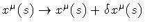
Another potential source of inequivalence stems from the fact that the
Nambu-Goto action is reparametrization invariant but non
linear with respect to the generalized velocity, whereas the Schild
action is linear but at the expense of reparametrization invariance. Apart
from all this, the standard procedure
to construct the path integral in quantum mechanics applies to
quadratic actions,
which is not the case for relativistic systems. One way to
deal with the problem would be to follow the Dirac
quantization procedure for constrained
systems. But then, a canonical evolution of the system
does not make sense because of the vanishing of the
Hamiltonian.
To preserve a Hamiltonian-type evolution, it is necessary to
start with a non-reparametrization invariant theory. Even in this
case, the resulting dynamics for an extended
object is non-canonical.
All of the above arguments converge to the focal question: if one
insists on a Hamiltonian, albeit non canonical formulation of string
dynamics, is there an evolution parameter which plays the role of
``time variable'', and is this choice consistent with
reparametrization invariance?
Previous attempts to deal with those questions lead to seemingly
conflicting conclusions. For instance, the string propagator
obtained in ref.[6], has been criticized in ref.[7].
From our vantage point, the critical issue is that of
reparametrization invariance. Both authors are led to a string
diffusion equation which is manifestly dependent on the string
parameter s, leaving us with the impression that the lack of
reparametrization invariance
of the classical action manifests itself even at the quantum
level. However, in ref.[6],
the physical Green function is obtained
by averaging over all the possible values of the proper
evolution parameter. In ref.[7], instead, it is
claimed that the parametric dependence of the propagation
kernel is only apparent
because the action is insensitive to the location of the area
increment along the world-sheet boundary.
The resulting wave equation is local, in the sense that
it is defined at a single, representative, point on the string loop, and
does not apply to the string as a whole. Evidently, in this approach
the string is treated as a collection of constituent points, and
this may well be a viable interpretation. However, inspired by our
previous work on the classical dynamics of p-branes [8],
[9], [10], we believe that the
dynamics of each individual point on the string does not give a
consistent account of the dynamics of the whole string.
The alternative point of view is that ``the whole string is
more than the sum of its parts'', and in this paper we wish to
suggest a different approach
which, in our view, addresses directly the question of the
choice of dynamical variables and the related issue of
reparametrization invariance in the classical theory as well as in
the quantum theory. The stipulation is also made that the
classical
theory must emerge as a well defined limiting case of the
quantum
theory. In order to fulfil this condition, we invoke a single
dynamical principle encompassing both areas of string-dynamics,
namely the Jacobi variational principle suitably adapted to the case
in which the physical system is a relativistic extended object.
Thus, the dynamical variables are restricted to vary within the
family of string trajectories which are solutions of the classical
equation of motion. In other words, the variational procedure
applies only to the final configuration of the string, rather than
to its spacetime history.
Against this conceptual backdrop, the formalism developed in
this paper, largely inspired by the work of Nambu
[11], [12] and Migdal [13], fully reflects
our emphasis on the global structure of the string: our action
functional is a reparametrized form of the
Schild action, manifestly invariant under general coordinate
transformation in the string parameter space, while preserving the
polynomial structure in the dynamical
variables; the natural candidate for the role of time
variable is the proper area of the string world-sheet
(equation (8)),
i.e., the invariant measure of the model manifold
representing
the evolution of the string. The final outcome is
a manifestly reparametrization
invariant Schrödinger equation which has the same form of
the corresponding equation obtained from the Nambu-Goto action
using a lattice approximation, and admits gaussian type
wave packets as solutions.
Our starting point is the Schild string action in Hamiltonian
form
where
 is the string tension,
  represents the model manifold of the string in parameter space, and
 represents its image in Minkowski space. Then,
 stands for the linear momentum canonically conjugated to
the world-sheet tangent element
stands for the linear momentum canonically conjugated to
the world-sheet tangent element
 .
Both variables were
originally introduced by Nambu [11],
[12]. More recently, the same variables were used to
formulate a gauge theory for the
dynamics of strings and higher dimensional extended objects
[8], [9], [10].
.
Both variables were
originally introduced by Nambu [11],
[12]. More recently, the same variables were used to
formulate a gauge theory for the
dynamics of strings and higher dimensional extended objects
[8], [9], [10].
In order to cast the action (2) in a reparametrization
invariant form, we introduce a new pair of world-sheet
coordinates
 through the
boundary preserving
transformation
through the
boundary preserving
transformation
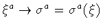 ,
and promote the original pair
,
and promote the original pair
 to the role of dynamical variables. Then,
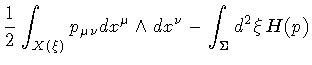
![$S [ x ( \xi ) , p ( \xi ) ]$](img19.gif) transforms into
transforms into
![\begin{displaymath}S [ x ( \sigma ) , p ( \sigma ) , \xi ( \sigma ) ]
=
\frac{...
...Sigma ( \sigma ) }
d \xi ^{a} \wedge d \xi ^{b}
\,
H(p)
.
\end{displaymath}](img20.gif) |
(3) |
The new action (3)
is numerically equivalent to (2) and leads to
the same equation of motion for  ,
.
Furthermore,
variation with respect to the new fields
,
.
Furthermore,
variation with respect to the new fields
 leads to the energy-balance equation
 |
(4) |
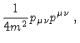
which, in our case, correctly shows that the Hamiltonian is
constant along a classical solution.
The action (3) is linear with respect to the ``velocities''
 and
and
 .
Hence, if one interprets
.
Hence, if one interprets
 as the momentum canonically conjugated to
,
then (3) acquires the form of a reparametrization invariant
theory in six dimensions [11].
as the momentum canonically conjugated to
,
then (3) acquires the form of a reparametrization invariant
theory in six dimensions [11].
The Jacobi equation for the string is obtained
by varying
![$S[ x ( \sigma ) , p ( \sigma ) , \xi ( \sigma ) ]$](img27.gif) within the family of world-sheets which solve the string
equations of motion.
We emphasize that this type of variation corresponds to a
deformation of the only
free boundary of the world-sheet, i.e. C, and corresponds
to the more familiar variation of the world-line end-point in the
case of a particle. Then, the steps leading to the Jacobi equation
are as follows. First, the contribution
from the variation of the world-sheet itself vanishes by
definition, and we obtain:
within the family of world-sheets which solve the string
equations of motion.
We emphasize that this type of variation corresponds to a
deformation of the only
free boundary of the world-sheet, i.e. C, and corresponds
to the more familiar variation of the world-line end-point in the
case of a particle. Then, the steps leading to the Jacobi equation
are as follows. First, the contribution
from the variation of the world-sheet itself vanishes by
definition, and we obtain:
![\begin{displaymath}\delta S _{\mathrm{cl.}}[ \partial X ; A]
=
\int _{\partial...
...
\,
\delta x ^{\mu}
-
H _{\mathrm{cl.}}
\delta A
\quad .
\end{displaymath}](img28.gif) |
(5) |
Next, we note that in view of the constancy of the Hamiltonian
over a classical trajectory, we can vary the area of the
domain without reference to
the specific point along the boundary
 where the
infinitesimal variation takes place. In other words, we can
move ``
where the
infinitesimal variation takes place. In other words, we can
move `` ''in front of the area integral and then trade the
functional variation
''in front of the area integral and then trade the
functional variation  for an ordinary differential
variation d A, and define
for an ordinary differential
variation d A, and define
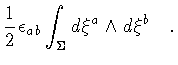
 |
(6) |
as the boundary momentum density. Similarly, the area-energy
density E can
be written as the partial derivative of the classical action
with respect to the invariant measure of the
domain
in parameter space:
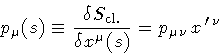
Hence, the Jacobi variational principle in the form of
equation (5)
shows that
 is conjugated to the spacetime
world-sheet boundary variation, while
H cl. describes the
response of the classical
action to an arbitrary area variation in parameter
space. Thus, if we consider string dynamics from the loop space
point of view [13], then A and
is conjugated to the spacetime
world-sheet boundary variation, while
H cl. describes the
response of the classical
action to an arbitrary area variation in parameter
space. Thus, if we consider string dynamics from the loop space
point of view [13], then A and
 can be
interpreted as the
``time'' and ``space'' positions of the final
string C
with respect to the initial one C 0, which we assume to be
fixed at the outset. In this perspective,
H cl. is the area-hamiltonian, or generator of the classical
evolution from the ``initial time'' T = 0 to the final time T = A.
Accordingly,
is the generator of
infinitesimal ``translations'' in loop space, which are
perceived as infinitesimal deformations
can be
interpreted as the
``time'' and ``space'' positions of the final
string C
with respect to the initial one C 0, which we assume to be
fixed at the outset. In this perspective,
H cl. is the area-hamiltonian, or generator of the classical
evolution from the ``initial time'' T = 0 to the final time T = A.
Accordingly,
is the generator of
infinitesimal ``translations'' in loop space, which are
perceived as infinitesimal deformations
 of the string shape in Minkowski space.
Finally, note that in this formulation, E represents the
energy per unit area associated with an extremal world-sheet
of the action (3), while
is the
momentum per unit length of the string loop C.
Therefore, the energy-momentum dispersion relation can be
written either as an equation between densities
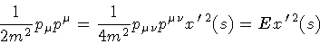 |
(9) |
or, as an integrated relation
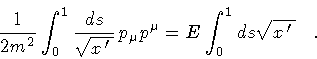 |
(10) |
The above equation, once written in terms of
S cl., turns into
the promised functional Jacobi equation for the string:
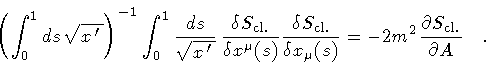 |
(11) |
Looking in more detail at this equation, we observe that the
covariant integration over s
takes into account all the possible locations
of the point, along the contour C,
where the variation can be applied. But, in this
way, every point of C is overcounted a ``number of times''
equal to the string proper length. The first factor, in
round parenthesis, is just the string proper length and removes such
overcounting. In other words, we sum over all the possible
ways in which one can deform the string loop, and then divide by the
total number of them. The net result is that
the l.h.s. of equation (11) is insensitive
to the choice of the point where the final string C is
deformed. Therefore the r.h.s. is a genuine
reparametrization
scalar which describes the system's response to the extent of
area variation, irrespective of the way in which the
deformation is implemented.
With hindsight, the wave equation proposed in
[6], [7] appears
to be more restrictive than equation (11), in the
sense that it
requires the second variation of the line fuctional
to be proportional to
 at any point on
the string loop, in contrast to equation (11) which represents
an integrated constraint on the string as a whole.
at any point on
the string loop, in contrast to equation (11) which represents
an integrated constraint on the string as a whole.
Equation (11) is the starting point in the first
quantization program via the Correspondence Principle:
one introduces the reparametrization invariant operators
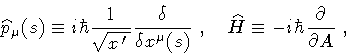 |
(12) |
and imposes the operatorial form of the
dispersion relation (10) on the string
wave functional
![$\Psi [ C ; A ]$](img43.gif) .
Alternatively, one can focus directly on
the string propagation kernel
.
Alternatively, one can focus directly on
the string propagation kernel
![$K \left[ x (s) , x _{0} (s) ; A \right]$](img44.gif) ,
in which case we turn to Feynman's
``sum over histories'' method since this is probably the
most natural and
effective way to define
in
quantum string-dynamics.
,
in which case we turn to Feynman's
``sum over histories'' method since this is probably the
most natural and
effective way to define
in
quantum string-dynamics.
Next: 3. Feynman and Jacobi
Up: String Propagator: a Loop
Previous: 1. Introduction
Stefano Ansoldi
Department of Theoretical Physics
University of Trieste
TRIESTE - ITALY