Next: 6. Conclusions
Up: 5. Computing the kernel
Previous: 5.1 Integrating the functional
5.2 Integrating the path integral
As a consistency check on the above result, and in order to
clarify some further
properties of the path integral, it may be useful to offer an
alternative derivation of equation (43) which is
based entirely on
the usual gaussian integration technique.
As we have seen in the previous section, the Feynman amplitude
can be written as follows
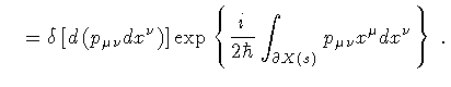
| |
|
![$\displaystyle K [ x (s) , x _{0} (s) ; A ]
=
\int _{ x _{0} (s)} ^{x (s)}
[D x ^{\mu} (\sigma)] [D p _{\mu \nu} (\sigma)] \times$](img111.gif) |
|
| |
|
 |
(44) |
In order to evaluate the functional integral (44), without
discretization of
the variables, we enlist the following equalities,
The functional delta function has support on the classical,
extremal trajectories of the string. Therefore, the momentum
integration is restricted
to the classical area-momenta and the residual integration
variables are the components
of the area-momentum along the world-sheet boundary
 .
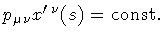
As a matter of fact, boundary conditions fix the initial and
final string loops C 0 and C but not the conjugate momenta.
In analogy to
the point particle case, the classical equations of motion on the
final world-sheet boundary
.
As a matter of fact, boundary conditions fix the initial and
final string loops C 0 and C but not the conjugate momenta.
In analogy to
the point particle case, the classical equations of motion on the
final world-sheet boundary
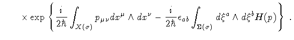
 |
(46) |
require that the three normal components of
 be constant, i.e.
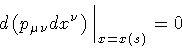
 Hence, the functional integral over the boundary momentum
reduces to a three dimensional, generalized, Gaussian integral
Hence, the functional integral over the boundary momentum
reduces to a three dimensional, generalized, Gaussian integral
![\begin{displaymath}\int [D p _{\mu \nu} (\sigma)]
\delta
\left[
d \left ( p _...
...
\right]
(\dots)
=
\int [d p _{\mu \nu}]
(\dots)
\quad .
\end{displaymath}](img119.gif) |
(47) |
Moreover, the Hamiltonian
is constant over a classical world-sheet and can be written
in terms of the boundary
.
In such a way,
the path integral is reduced to the Gaussian integral over the
three components of
which are normal to the boundary
| K [ x (s) , x 0 (s) ; A ] |
 |
![$\displaystyle \mathcal{N} \! \!
\int \! [d p _{\mu \nu}] \!
\exp \!
\left\{ \!
...
...) d x ^{\nu}
-
\frac{A}{4 m ^{2}}
p _{\mu \nu}
p ^{\mu \nu}
\right] \!
\right\}$](img121.gif) |
|
| |
|
![$\displaystyle \mathcal{N} \! \!
\int \! [d p _{\mu \nu}] \!
\exp \!
\left\{ \!
...
... - C _{0}]
-
\frac{A}{4 m ^{2}}
p _{\mu \nu}
p ^{\mu \nu}
\right] \!
\right\}
,$](img122.gif) |
|
and correctly reproduces the expression
(43).
Next: 6. Conclusions
Up: 5. Computing the kernel
Previous: 5.1 Integrating the functional
Stefano Ansoldi
Department of Theoretical Physics
University of Trieste
TRIESTE - ITALY
![$\displaystyle \int _{x _0 (s)} ^{x (s)} [D x ^{\mu} (\sigma)]
\exp
\left\{
\fra...
...bar}
\int _{X (\sigma)}
p _{\mu \nu} \, d x ^{\mu} \wedge d x ^{\nu}
\right\}
=$](img113.gif)
![$\displaystyle \quad =
\int _{x _0 (s)} ^{x (s)} [D x ^{\mu} (\sigma)]
\exp
\lef...
...gma)} \! \! \! \!
x ^{\mu} \, d p _{\mu \nu} \wedge d x ^{\nu}
\right]
\right\}$](img114.gif)