5.2 Approximating the action

To get some analytical result we try to fit the $20000$ points for which we evaluated the action with some simple (polynomial) function. In this way we will be able to get an (approximated) relation among $Q$, $H$ and $n$. The choice of the approximating function is done with two goals in mind:

1. to approximate in the best possible way the behaviour of the action $\bar{S}$ at least in some regime;
2. to have a simple enough expression to get an algebraic relation among $Q$, $H$ and $n$.

To fulfill the above requirements we first analyze the leading $\Theta$ dependence of the action $\bar{S}$, expressed as the integral (24). From E we se that $\bar{P} (x) \sim x ^{2} + {\mathcal{O}} (x) ^{2}$ and the upper turning point $x _{\mathrm{min}} (\Theta) \sim \Theta + {\mathcal{O}} (\Theta)$, so that $\bar{S} (\Theta) \sim \Theta ^{3} + {\mathcal{O}} (\Theta) ^{3}$. We thus choose an approximating function starting with a third power of $\Theta$ and having the next two powers of $\Theta$:

$$A x ^{5} + B x ^{4} + C x ^{3} ,$$ (27)

The coefficients $A$, $B$, $C$ in (27) have been determined from the $20000$ sample points using the function Regress of Mathematica$^{\circledR}$, with the parameter IncludeConstant $\to$ False, since there is no constant term in the model: they result to be, together with the corresponding standard errors,

$$A = + 10.11 \pm 0.04$$

$$B = - 7.39 \pm 0.04$$ (28)

$$C = + 3.64 \pm 0.01 ,$$

with an adjusted regression coefficient of $0.99981$.
The comparison between approximated and numerical evaluated actions is plotted in figure 12.

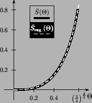
Figure: Comparison between approximated and numerical evaluated actions. The expression $\bar{S} _{\mathrm{reg.}} (\Theta)$ is obtained, as described in the text, by a fit to a suitable polynomial. This figure aims to show that the main behaviour can be qualitatively approximated, but must not be taken to imply that the approximation is everywhere very good. Indeed when the action is very small, a very small approximation error can still give a relevant relative uncertainty.

Level curves of the approximated action are plotted in figure 13.

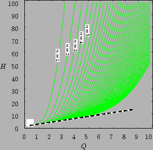
Figure 13: Graph of the level curves for the approximated action levels $1 , 2 , \dots , 50$. The levels are obtained using the approximating polynomial action with the function ContourPlot of Mathematica$^{\circledR}$. The thicker dashed black line displays the limit $H = (4/3) ^{3/2} Q$ of the condition $Q / H > (3/4) ^{3/2}$ for which bounded trajectories exist.

From the approximated expression (27), which by (25) and (26) must equal $n$ when multiplied by $H ^{2}$, we can get the following equation of the third degree in H,

$$A Q ^{5} + B Q ^{4} H + C Q ^{3} H ^{2} - n H ^{3} = 0 :$$ (29)

this can be solved exactly to get the approximated relation for $H$ as a function of $Q$ and $n$ as it comes from the simplified expression (27) for the action. The quite complex algebraic expression is

$$H (Q ; n) = \frac{C Q ^{3}}{3 n} + \frac{2 ^{1/3} H _{1} (Q ; n) Q ^{7/3}} {3... ...3]{H _{2} (Q ; n) + \sqrt{4 Q ^{2} H _{1} ^{3} (Q ; n) + H _{2} ^{2} (Q ; n)}}}$$

$$\qquad - \frac{Q ^{5/3}\sqrt[3]{H _{2} (Q ; n) + \sqrt{4 Q ^{2} H _{1} ^{3} (Q ; n) + H _{2} ^{2} (Q ; n)}}}{2 ^{1/3} 3 n} ,$$ (30)

where

$$H _{1} (Q ; n) = - C ^{2} Q ^{2} - 3 B _{1} n$$

$$H _{2} (Q ; n) = - 2 C ^{3} Q ^{4} - 9 B C n Q ^{2} - 27 A ^{2} n ^{2}$$

and the approximated relations above are only valid if

$$H > \frac{\vert Q \vert}{(3/4) ^{3/2}} ,$$

a condition plainly coming from (23). The approximated levels of figure 13 are nothing but the graphs of the $n = \mathrm{const.}$ relations coming from (30).