Next: 5. The Coleman-Weinberg mechanism
Up: Membrane Vacuum as a
Previous: 3. The action
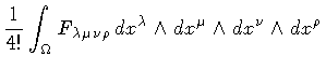
The action (8) leads to the pair of coupled field equations
which describe the interaction between the membrane field and the
 gauge potential. Now, we wish to show that the superconducting membrane
condensate contains regions of spacetime, or bags of non
superconducting vacuum.
gauge potential. Now, we wish to show that the superconducting membrane
condensate contains regions of spacetime, or bags of non
superconducting vacuum.
Recall that in a type-II superconductor the magnetic field is
confined by the superconducting
vacuum pressure within a string-like flux tube. Similarly,
the membrane condensate confines the gauge field strength within
a membrane-like boundary layer surrounding a region of ordinary
vacuum. Indeed, in analogy with the superconducting solution of
scalar QED, we assume the following asymptotic boundary condition for
![$\Psi [S]$](img5.gif)
![\begin{displaymath}\Psi [S]
\equiv
\frac{\phi}{g ^{2}}
e ^{i \displaystyle{\...
...} d x ^{\mu} \wedge d x ^{\nu}
\theta _{\mu \nu} (x)
\right)
\end{displaymath}](img70.gif) |
(21) |
where  is a constant.
This is the form of the membrane field when the three volume
enclosed by S is much larger than the three volume of the vortex
spacetime image. Then, from equation (19) we obtain the corresponding
asymptotic form of
:
is a constant.
This is the form of the membrane field when the three volume
enclosed by S is much larger than the three volume of the vortex
spacetime image. Then, from equation (19) we obtain the corresponding
asymptotic form of
:
![\begin{displaymath}\left(
\frac{\delta}{\delta \sigma ^{\mu \nu \rho} (s)}
-
...
... \rho} =
\frac{1}{g}
\partial _{[ \mu}
\theta _{\mu \nu ]}.
\end{displaymath}](img72.gif) |
(22) |
Therefore, the flux of
 across a large four dimensional region
 enclosing B is given by
Thus, the physical consequence of the monodromy of
is that the flux of
through a region enclosing B
is quantized in units of  .
.
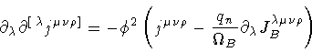
In the superconducting phase, equation (20) becomes
![\begin{displaymath}\partial _{\lambda}
F ^{\lambda \mu \nu \rho} (x)
=
-
\ph...
...a ^{\nu \rho ]} (x)
\right)
\equiv
-
j ^{\mu \nu \rho} (x)
\end{displaymath}](img79.gif) |
(24) |
in which we have introduced the supercurrent density
 .
Equation (24) holds only where
.
Equation (24) holds only where
 is a regular function. In the domain of singularity,
where the partial derivatives of
do not commute,
the covariant curl of
is a regular function. In the domain of singularity,
where the partial derivatives of
do not commute,
the covariant curl of
![$\partial ^{[ \, \mu} \theta ^{\nu \rho]} (x)$](img82.gif) should be interpreted in the
sense of distribution theory. Indeed, if we apply the covariant curl
operator to both sides of equation (24), we obtain
should be interpreted in the
sense of distribution theory. Indeed, if we apply the covariant curl
operator to both sides of equation (24), we obtain
![\begin{displaymath}\partial ^{[ \, \lambda}
j ^{\mu \nu \rho ]}
=
-
\phi ^{2...
...[ \, \lambda}
\partial ^{\mu}
\theta ^{\nu \rho ]}
\right)
\end{displaymath}](img83.gif) |
(25) |
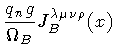
The last term in (25) may not be disregarded without violating
(7). Therefore in order to match (23) with (7),
we define
where,
 and
and
 are, respectively, the bag four-volume and the bag current.
Thus, the supercurrent can be determined from the equation
are, respectively, the bag four-volume and the bag current.
Thus, the supercurrent can be determined from the equation
 |
(27) |
by means of the Green function method:
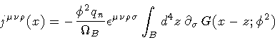 |
(28) |
where
G ( x - z ) is the scalar Green function
![\begin{displaymath}\left[
\partial ^{2}
+
\phi ^{2}
\right]
G ( x - z ; \phi ^{2})
=
\delta ^{4)} ( x - z )
.
\end{displaymath}](img91.gif) |
(29) |
Then, from equation (20), (25) and
(28), we find the form of the confined gauge field
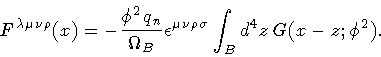 |
(30) |
The analogy between the membrane vacuum and a type-II
superconductor now seems manifest: in the ordinary vacuum
does
not propagate any degree of freedom.
Rather, it corresponds to a uniform energy background. However, in
the superconducting phase
becomes a dynamical field describing
a massive, spin-0 particle [10]. The source for the massive
field is the bag current (26). In a boson particle
condensate, the magnetic
field is confined to a thin flux tube surrounding the vortex line;
in the membrane condensate, the
-field is confined within the membrane
which encloses the ordinary vacuum bag. The gauge field
provides the ``skin'' of the bag. To complete the analogy, in the
next section we show that the thickness
of the membrane is given by the inverse of the
dynamically generated mass of
.
Next: 5. The Coleman-Weinberg mechanism
Up: Membrane Vacuum as a
Previous: 3. The action
Stefano Ansoldi
Department of Theoretical Physics
University of Trieste
TRIESTE - ITALY
![$\displaystyle {\langle}
\Big \vert
\left(
\frac{\delta}{\delta \sigma ^{\mu \nu \rho} (s)}
-
i
g
A _{\mu \nu \rho} \right)
\Big \vert ^{2}
\Psi[S]
{\rangle}$](img67.gif)
![$\displaystyle \frac{1}{3! g}
\oint _{\Gamma} d x ^{\mu} \wedge d x ^{\nu} \wedg...
...tial _{[ \mu}
\theta _{\nu \rho ]}
=
\frac{2 \pi n}{g}
\qquad
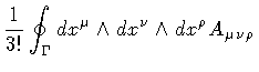
n = 1 , 2 , \dots$](img77.gif)
![$\displaystyle \frac{q _{n} g}{\Omega _{B}}
\epsilon ^{\lambda \mu \nu \rho}
\int _{B} d ^{4} \xi \,
\delta ^{4)}
\left[ x - z( \xi ) \right]$](img85.gif)