The WWM relation establishes a one-to-one correspondence between a linear
operator,
![]() in our case, acting over a Hilbert
space
in our case, acting over a Hilbert
space ![]() of square integrable functions on
of square integrable functions on ![]() , and a
smooth function
, and a
smooth function
![]() which is the anti-Fourier
transform of
which is the anti-Fourier
transform of
![]() in (5):
in (5):
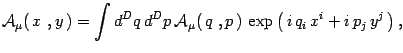
![$\displaystyle {\cal A}_\mu(\, q\ , p\,)={1\over N}Tr_{{\cal H}}
\left[\, {\mbox...
...oldmath {$p$}}}_i\, q^i -i\,
{\mbox{\boldmath {$q$}}}_j\, p^j\,\right)\right]\ $](img51.gif) |
(7) |
 |
(8) |
 |
|||
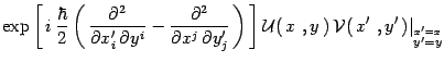
![$\displaystyle \exp\left[\, i\, {\hbar\over 2}\,\omega^{ab} \,
{\partial^2\over ...
... \xi^b } \,
\right]{\cal U}(\,\sigma\,)\, {\cal V}(\,\xi\,)
\vert_{\sigma=\xi},$](img58.gif) |
(9) |
| (10) |
![$\displaystyle {1\over \hbar}\, \left[\, {\mbox{\boldmath {$A$}}}\ ,
{\mbox{\boldmath {$A$}}}\,\right]\rightarrow
\left\{\, {\cal U}\ , {\cal V}\,\right\}_{MB}$](img66.gif) |
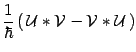 |
||
| (11) |
| (12) |
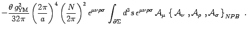
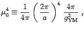
The last step of the mapping between matrix theory into a field model is carried
out through the identification of the ``deformation parameter'' ![]() with the inverse of
with the inverse of ![]() :
:
| (14) |
After this technical detour, let us come back to the two terms
in the reduced action (2) which are mapped by the WWM
correspondence into
We could also write equation (16) without the ![]() -product
between the two Moyal brackets, due to the following property of integration
over phase space in the absence of boundary
[12],
-product
between the two Moyal brackets, due to the following property of integration
over phase space in the absence of boundary
[12],
![]() .
Extra terms will appear whenever boundaries are present
[13].
This is just what we expect to find, thus, we shall keep the
.
Extra terms will appear whenever boundaries are present
[13].
This is just what we expect to find, thus, we shall keep the ![]() -product
in (16) .
-product
in (16) .
Before discussing the case ![]() , it can be useful to show as the classical
limit of
, it can be useful to show as the classical
limit of
![]() , with
, with ![]() is related to the action
of a bosonic string, which for simplicity we assumed to closed. Thus, only
the term
is related to the action
of a bosonic string, which for simplicity we assumed to closed. Thus, only
the term
![]() has to be taken into
account and gives:
has to be taken into
account and gives:
|
brane Fields
|
Symmetry
|
|
|---|---|---|
|
|
|
Reparametrization
Conformal Invariance |
|
|
|
Volume Preserving
Diffeomorphisms |
|
|
|
Reparametrization
Invariance |
|
|
Reparametrization
Invariance |
|
| Table 1: This table summarizes the various actions for the bulk three-brane and boundary two-brane we used in the paper. | ||
Moving to the case ![]() , it can be useful to recall that
the action for a
, it can be useful to recall that
the action for a ![]() -brane can be written in several different forms
[16]. With hindsight, we need to recall
the conformally invariant four dimensional
-brane can be written in several different forms
[16]. With hindsight, we need to recall
the conformally invariant four dimensional ![]() -model action
introduced in [17]
-model action
introduced in [17]
In equation (19) the indices inside square roots are
anti-symmetrized and
target spacetime indices are saturated by a flat metric ![]() .
In this
.
In this ![]() model approach
model approach ![]() would be the coordinates of a
would be the coordinates of a ![]() -brane
in four dimensional target spacetime and the
-brane
in four dimensional target spacetime and the ![]() are coordinates
on the
are coordinates
on the ![]() -dimensional world volume. Moreover,
-dimensional world volume. Moreover,
![]() is the
flat Minkowski metric tensor in target spacetime, while
is the
flat Minkowski metric tensor in target spacetime, while
![]() is an independent, auxiliary, world-volume metric providing reparametrization
invariance of the model. It can be worth to remind that,
once the auxiliary metric is algebraically solved in terms of the induced
metric, i.e.
is an independent, auxiliary, world-volume metric providing reparametrization
invariance of the model. It can be worth to remind that,
once the auxiliary metric is algebraically solved in terms of the induced
metric, i.e.
![]() , then,
, then,
![]() turns into a Nambu-Goto type action. But, the Nambu-Goto action
for a
turns into a Nambu-Goto type action. But, the Nambu-Goto action
for a ![]() -brane embedded in a four dimensional target spacetime is nothing
but the world volume of the brane itself. Accordingly,
the constant
-brane embedded in a four dimensional target spacetime is nothing
but the world volume of the brane itself. Accordingly,
the constant ![]() in front of it can be identified with the
(constant) pressure inside the bag. Despite its non-trivial look,
in front of it can be identified with the
(constant) pressure inside the bag. Despite its non-trivial look,
![]() does not describe transverse, propagating degrees of freedom, but
only a constant energy density and pressure, non-dynamical, spacetime domain.
All the dynamics is carried by the boundary of the domain, in a way which
seems to satisfy the holographic principle
[19] in a very
strict sense: all the non-trivial dynamical degrees of freedom are confined to
the
membrane enclosing the bag. Among various kind of relativistic membranes the
Chern-Simons one is a very interesting objects
[18].
In the action
does not describe transverse, propagating degrees of freedom, but
only a constant energy density and pressure, non-dynamical, spacetime domain.
All the dynamics is carried by the boundary of the domain, in a way which
seems to satisfy the holographic principle
[19] in a very
strict sense: all the non-trivial dynamical degrees of freedom are confined to
the
membrane enclosing the bag. Among various kind of relativistic membranes the
Chern-Simons one is a very interesting objects
[18].
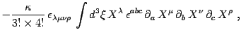
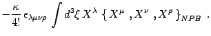
In the action ![]() the three-volume element of the membrane is represented
by the Nambu-Poisson brackets, while
the three-volume element of the membrane is represented
by the Nambu-Poisson brackets, while ![]() is a constant
with dimensions of energy per unit three-volume. The presence of the
Nambu-Poisson bracket suggests a new kind of formulation of both
classical and quantum mechanics for such an object,
which is worth investigating by itself [20].
is a constant
with dimensions of energy per unit three-volume. The presence of the
Nambu-Poisson bracket suggests a new kind of formulation of both
classical and quantum mechanics for such an object,
which is worth investigating by itself [20].
The formal structures of (16), (17) and
(19), (20)
are so similar that one expects some kind of relationship among these
actions. On the other hand, we notice that while the
![]() action
is defined over a flat phase space,
action
is defined over a flat phase space, ![]() involves integration
over a curved world-volume. In the latter case a Moyal deformation
would be no longer valid, due to the lack of associativity of the
involves integration
over a curved world-volume. In the latter case a Moyal deformation
would be no longer valid, due to the lack of associativity of the
![]() -product, and a Fedosov deformation quantization would be required
[21]. However, the Weyl symmetry of the
-product, and a Fedosov deformation quantization would be required
[21]. However, the Weyl symmetry of the ![]() suggests to
restrict5the world metric to the conformally flat sector:
suggests to
restrict5the world metric to the conformally flat sector:
| (22) |
The alleged correspondence between
![]() and
and
![]() is clear.
By choosing
is clear.
By choosing ![]() in (16), we find
in (16), we find
By rescaling the fields according with6
 |
(27) |
 |
(28) |
 |
|||
 |
(29) |
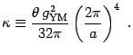
As a consistency check of our dynamically generated bag pressure
consider equation (30) in the strong coupling regime,
where it is conventionally assumed
![]() .
If we identify the inverse lattice spacing
.
If we identify the inverse lattice spacing ![]() with the
with the ![]() scale
scale
![]() then, equation (30)
provides
then, equation (30)
provides
The actual value of ![]() is close to
is close to ![]() ; this is not a bad result, compared with the phenomenological
value
; this is not a bad result, compared with the phenomenological
value
![]() , if one takes into account the uncertainty on the
value of
, if one takes into account the uncertainty on the
value of ![]() , i.e.
, i.e.
![]() .
.
 |
||
|
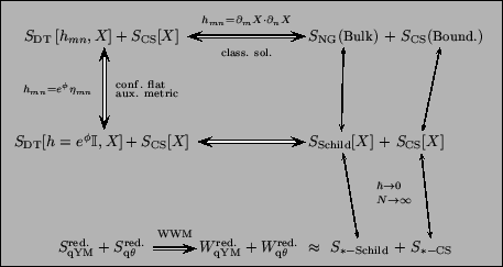
Figure 1: The figure shows the web
of relationships among the various actions discussed in this note. It
can be read as ``map'' to move from the Yang-Mills action, in the lower
left corner, to complete bag action in the upper right corner.
|
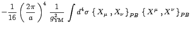
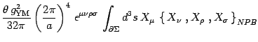
||
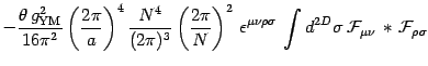
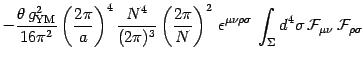
![$\displaystyle -{1\over 16}\left({2\pi\over a}\right)^4
{\left({N\over 2\pi}\rig...
...[\, m}\, {\cal A}^{\mu}\circ \partial_{n\, ]}\, {\cal A}^{\nu}\,
\omega^{mn}\ ,$](img80.gif)
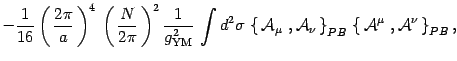
![$\displaystyle -{ \theta\, g^2_{\mathrm{YM}} \over 64\pi^2}
\left({2\pi\over a}\...
...\, m}{\cal A}_{\rho}\circ \partial_{n\, ]}\, {\cal A}_{\sigma}\,
\omega^{mn}\ .$](img83.gif)
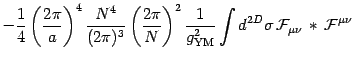
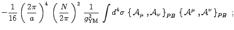
![$\displaystyle -{1\over 16}
\left(\, {2\pi\over a}\,\right)^4
{N^4\over (2\pi)^4...
...ega^{mn} \,
\partial_{[\, m}\,{\cal A}^{\mu}\, \partial_{n\,]}\,
{\cal A}^{\nu}$](img89.gif)
![$\displaystyle -{1\over 16}
\left(\, {2\pi\over a}\,\right)^4
\, \left(\, { N\ov...
...mega^{mn} \,
\partial_{[\, m}\,{\cal A}^{\mu}\,\partial_{n\,]}\,
{\cal A}^{\nu}$](img119.gif)
![$\displaystyle -{ \theta\, g^2_{\mathrm{YM}} \over 64\pi^2}
\left({2\pi\over a}\...
...rtial_{m}\, {\cal A}_{\rho}\, \partial_{n}\, {\cal A}_{\sigma}\,
\omega^{mn\,]}$](img122.gif)