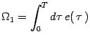
Following exactly the same steps as in the previous case, we obtain
| (13) | |||
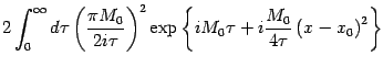
| (14) | |||
| (15) | |||
 |
(16) | ||
| (17) |
 |
|||
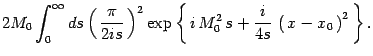 |
(18) |
Returning now to the general case, one may
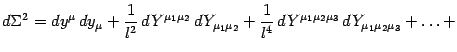
regard the expression (1) as the propagator of a poly-brane, i.e., a generic ![]() -brane combined with its baricentric
coordinate, moving in a spacetime with metric:
-brane combined with its baricentric
coordinate, moving in a spacetime with metric:
As a mathematical construct, the line element (20) has long been
known at least to some practitioners of Clifford algebras. For instance,
Pezzaglia has introduced it to discuss the long standing problem of a
classical spinning particle [11]. In that classical context, Eq.
(20) may be interpreted as an extension of the usual Lorentzian
line element.
To our mind, however, the Clifford line element establishes a mathematical
and physical link between the theory of relativistic extended objects, as
developed over the years by the authors, and the very structure of
spacetime geometry at the Planck scale. Indeed, the whole cardinal
concept of relativity of motion may be extended to the broader
context of relativity of dimensions. By ``relative dimensionalism'',
we mean that the new Clifford metric opens the possibility of (generalized
Lorentz) transformations between different ![]() -branes, so that their
effective dimensionality, and the very geometry of spacetime, become resolution dependent.
-branes, so that their
effective dimensionality, and the very geometry of spacetime, become resolution dependent.
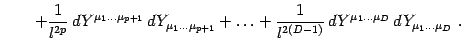
In order to substantiate this connection between the Clifford line element
and the short distance structure of spacetime, note that the generalized
Lorentzian metric (20) calls for
the introduction of a fundamental length, ![]() , or energy scale
, or energy scale ![]() ,
in the fabric of spacetime, so that, what is described as a scalar, vector,
bivector, or
,
in the fabric of spacetime, so that, what is described as a scalar, vector,
bivector, or ![]() -vector, becomes now observer dependent. In the
language of
-vector, becomes now observer dependent. In the
language of ![]() -branes, the same fundamental length is necessary in order
to include in the line element (20) an ``areal distance'', playing
the role of time for each kind of
-branes, the same fundamental length is necessary in order
to include in the line element (20) an ``areal distance'', playing
the role of time for each kind of ![]() -brane, so that, what is physically
perceived as a point, world-line, world-sheet, or
-brane, so that, what is physically
perceived as a point, world-line, world-sheet, or ![]() -brane really
depends on the resolving power of the Heisenberg microscope used to probe
the short distance structure of spacetime.
-brane really
depends on the resolving power of the Heisenberg microscope used to probe
the short distance structure of spacetime.
In order to clarify the physical meaning of ![]() , let us consider
the new tension-shell condition defined by
the vanishing of the denominator in Eq. (1):
, let us consider
the new tension-shell condition defined by
the vanishing of the denominator in Eq. (1):
|
|
(22) | ||
 |
(23) |
| (25) |
| (29) |
| (32) |
The standard procedure, at this point, is to minimize the position uncertainty
| (34) |
By switching once again to natural units, ![]() , we see that the
minimum uncertainty, or quantum of resolution is proportional to the
length scale
, we see that the
minimum uncertainty, or quantum of resolution is proportional to the
length scale ![]() , i.e.
, i.e.
According to the fundamental condition (35), strings, or any
![]() -brane, or test body for that matter, cannot probe distances shorter
than
-brane, or test body for that matter, cannot probe distances shorter
than ![]() . Thus, the length scale
. Thus, the length scale ![]() , originally introduced in the
line element (20) for purely dimensional reasons, can now be given
the meaning of a minimum universal length5.
, originally introduced in the
line element (20) for purely dimensional reasons, can now be given
the meaning of a minimum universal length5.
![\begin{displaymath}
{d ( \Delta x) \over d ( \Delta k_x)}=0\ \Longrightarrow
\le...
...eft[\, {2\over (2p-1)\,
l_{Pl}^{2p}\,
\beta}\, \right]^{1/p}
,
\end{displaymath}](img74.gif)