In the second part of this note we shall discuss the above equivalence
at the quantum level. The basic quantity encoding the -brane
quantum dynamics is the boundary wave functional, or
vacuum--one-brane amplitude
(10)
where the sum is over all bulk fields configurations inducing
``hatted'' fields on the boundary of the brane. We are assuming
that the brane world manifold has a single, -dimensional boundary,
parametrized as
,
,
which is mapped into the physical brane
;
and are the induced metric and gauge
potential over
.
The integration variables in ``live'' in the brane bulk,
while we let free the fields induced on the boundary, i.e. we do
not assign an independent classical action to the hatted fields.
The first field to be integrated out is the gauge -form . The
standard routine goes through a lengthy procedure of gauge fixing
and Fadeev-Popov compensation to invert the classical kinetic
operator and define an appropriate quantum propagator.
On the other hand, one knows that
a gauge -form over a -dimensional manifold has no dynamical
degrees of freedom and can describe only a static interaction.
In such a limiting case the Fadeev-Popov procedure leaves no
propagating degree of freedom at the quantum level. To shorten
the whole gauge fixing procedure of ghost terms with different rank
[9], we shall provide an alternative ``recipe'' to kill all
the apparent degrees of freedom. We write the path-integral in the
first order version, where the gauge
potential and field strength are introduced as independent
integration variables [10] and we integrate away the
gauge part of after inserting gauge fixing Dirac delta's and the
corresponding ghost determinants in the functional measure.
The remaining, gauge invariant part of enforces to
be a classical solution of the field equations, which is a constant
background field. No propagating degrees of freedom
survive at the quantum level. A formal proof of the
equivalence between second order and first order quantization
procedures, in the general case of a -form in dimensions,
is beyond the purpose of this short note. Rather,
we will briefly consider the simplest, non trivial case which is
gauge form over a two-dimensional, flat manifold without
boundary,
and then translate the result to the case we are studying.
The first order, gauge fixed and Fadeev-Popov compensated path
integral is
(11)
By splitting into the sum of a ``transverse'' vector
and a ``gauge part''
, the integration measure turns into
and (11) reads
(12)
where the the gauge part has been integrated away
thanks to the Fadeev-Popov determinant
and
only the gauge invariant vector remains in the classical action.
The extra Jacobian, coming from the change of the
integration measure, will be cancelled in a while when integrating .
The pay off for relaxing the relationship between
and and getting rid of the gauge part is that linearly enters the first
order action, i.e. plays the role of Lagrange
multiplier imposing to satisfy the classical field equations
(13)
Equation (13) shows that the first order formulation
of a limiting rank, abelian gauge theory, and
the Fadeev-Popov prescription lead to a ``trivial'' path
integral for .
The Dirac-delta picks up the classical configurations of
the world tensor and the whole path-integral ``collapses''
around the classical trajectory5.
Thus, is ``frozen'' to a constant value and no degrees of
freedom are left free to propagate.
The same result can be obtained, with some additional work,
for as well. Accordingly, we get
(14)
The first term in (14) is a pure boundary quantity produced
by a partial integration of the term
.
A similar term arises in string theory when boundary and bulk quantum
dynamics are properly split [11].
After integrating out the gauge degrees of freedom the resulting
path-integral reads
(15)
We remark that this integration procedure is exact and
leads to a bulk action plus a boundary correction represented
by the generalized Wilson factor
.
We also notice that the world metric enters the path-integral only
through
the world volume density. Accordingly, we can ``change'' integration
variable
The saddle point value for the auxiliary field is defined
by:
(18)
By expanding around the saddle point
we obtain the Dirac-Nambu-Goto path-integral. Correspondingly,
we get the following semi-classical equivalence relation
![$\displaystyle \int[ DF ] [ DA^T ] [ D\phi ]
\left( \det\Box \right)^{1/2}
\delta\left[ \Box\phi \right]
\times$](img66.gif)
![$\displaystyle \qquad \qquad \times
\Delta_{FP}\exp\left\{ i\int d^2\sigma \left...
...n}
F^{mn}-{1\over 2}F^{mn} \partial_{[ m} A^T_{n ]} \right]
\right\}$](img67.gif)
![$\displaystyle \int [ DF ][ DA^T ]
\left( \det\Box \right)^{1/2}
\ex...
...{mn}
F^{mn}+{1\over 2}A^T_n \partial_m F^{mn} \right] \right\}
\quad ,$](img68.gif)
![$\displaystyle \int[ DF ] \left( \det\Box \right)^{1/2}
\delta\left[ \...
...\exp\left\{ i\int d^2\sigma \left[ {1\over 4}F_{mn}
F^{mn} \right] \right\}$](img71.gif)
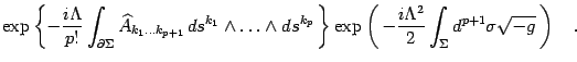
![$\displaystyle \int[ DF ]
\delta\left[ F^{mn}-\Lambda \epsilon^{mn} \ri...
...t\{ i\int d^2\sigma \left[ {1\over 4}F_{mn}
F^{mn} \right] \right\}
\quad .$](img72.gif)
![$\displaystyle \qquad \quad \times \int [ DF] \left( \det\Box \right)^{1/...
...rtial_{m_1 }\left( \sqrt{-g}
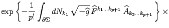
F^{m_1 m_2\dots m_{p+1}} \right) \right]\times$](img76.gif)
![$\displaystyle \int^{\widehat g} [ Dg_{mn} ]
\int^{\widehat Y} [ DY^\mu ]
...
...hat
A_{k_1\dots k_{p+1}} ds^{k_1}\wedge \dots\wedge ds^{k_p} \right)
\times$](img80.gif)
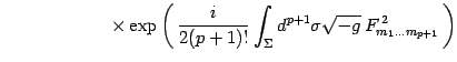
![$\displaystyle \qquad\qquad\times\exp\left( -i\int_\Sigma d^{p+1}\sigma \left[...
... 2} {(-\gamma)\over \sqrt{-g}}
+{\Lambda^2\over 2}\sqrt{-g} \right] \right)$](img81.gif)
![$\displaystyle \int^{\widehat g} [ Dg_{mn} ] \int^{\widehat Y}
[ DY^\mu ]\...
...-\gamma)\over \sqrt{-g}}
+{\Lambda^2\over 2}\sqrt{-g} \right] \right)
\quad .$](img83.gif)
![\begin{displaymath}
Z=\int^{\widehat e} [ De ] \int^{\widehat Y} [ DY^\mu...
...gma)}
+{\Lambda^2\over 2} e(\sigma) \right] \right)
\quad .
\end{displaymath}](img86.gif)
![$\displaystyle \int^{\widehat g} [ Dg_{mn} ] \int^{\widehat Y} [ DY^\mu ]
\int^{\widehat A}[ DA ]\times$](img90.gif)
![$\displaystyle \qquad\qquad\times\exp\left[ -i m_{p+1} \int_\Sigma d^{p+1}\sig...
...int_\Sigma
d^{p+1}\sigma
\sqrt{- g}
F_{m_1\dots m_{p+1}}^{ 2}(A) \right]$](img91.gif)
![$\displaystyle \int [ DY^\mu ] W_{\widehat A}
[ \partial\Sigma ]\exp\left[ - i\rho_p
\int_\Sigma d^{p+1}\sigma \sqrt{-\gamma} \right]
\quad .$](img93.gif)