Index
Chapter 1
Motivations
In this report we want to predict the approach to equilibrium of a spherically symmetric
field-particle system initially excited in a non-equilibrium state where the particle is in an
unstable circular orbit around the origin [1].
In particular we will be concerned with the realization of a quasistatic approximation
to the exact dynamical problem. As the newly built gravitational wave detectors are
preparing to receive their first set of data, theorical efforts are being carried on to solve
exactly Einstein’s equation to be able to timely interpret such data. Our quasistatic
approximation co is in an unstable circular orbit could become an important tool in the
event that such theoretical efforts fail to solve the exact problem in time. The
approximation should be particularly usefull in interpreting the waveform coming from
slowly decaying binary neutron stars.
Binary neutron stars are known to exist and for some of the systems in our own
galaxy (like the relativistic binary radio pulsar PSR B1913+16 and PSR B1534+12)
general relativistic effects in the binary orbit have been measured to high precision. With
the construction of laser interferometers well underway, it is of growing urgency that we
be able to predict theoretically the gravitational waveform emitted during the inspiral and
the final coalescence of the two stars. Relativistic binary systems, like binary neutron
stars and binary black holes pose a fundamental challange to theorists, as the
two-body problem is one of the outstanding unsolved problems in classical general
relativity.
Chapter 2
Introduction
When studying a two body problem one decomposes it in the trivial problem involving
the center of mass motion and the harder one involving the relative motion of the two
masses. Is the second one, we want to focus on. Since we don’ t want to deal with all the
difficulties of General Relativity (there is no analytic solution to the two body problem in
GR) and we want to have a more realistic theory than the Newtonian one, we
choose to employ a theory which describes gravitation by a nonlinear scalar
gravitational field Φ in special relativity. To decribe the relative motion in a two body
problem we just need one particle moving around the origin. The particle motion is
confined at all times in its orbital plane, and its position there is determined by the
distance from the origin rp, and the azimuthal angle ϕp. To follow the dynamical
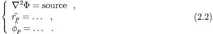
evolution of the field-particle system in scalar gravity, one needs to solve a single
hyperbolic partial differential equation describing the field evolution, coupled to a
system of two ordinary differential equations describing the particle motion,
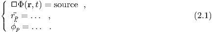
The source term of the field equation is where the coupling between the field and the
particle dynamics takes place, and is responsible for the nonlinearity of the problem:
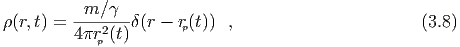
source ~ exp(Φ)ρ, where ρ(r,t) = (m∕γ)δ(r - rp(t)) is the comoving matter density, m
the particle rest mass, and γ the Lorentz factor.
In particular we want to study the even simpler, spherically symmetric problem. It is
infact a peculiarity of scalar gravitation that of being able to generate gravitational
waves even in spherical symmetry. This allows the study of wave generation and
propagation with the use of just one spatial dimension plus time. In spherical
symmetry the particle angular momentum ũϕ is conserved. There are then three
important quantities in our problem: the initial distance from the origin ri,
the particle rest mass m, and its angular momentum ũϕ. Two adimensional
combinations of these quantities are particularly important to parametrize the
problem:
-
(1)
- The initial compaction α = ri∕m which tunes the nonlinearity of the problem:
-
α ≫ 1
- The system is in a weak field and slow particle velocity regime.
Newtonian gravitation provides a good analytical approximation to the
nearly linear and periodic system.
-
α ~ 1
- The system is nonlinear and aperiodic. There is no analytic solution to
the coupled equations (2.1), and a numerical integration is needed. In this
report we will describe an approximate solution which works well when
the system relaxes slowly.
-
(2)
- An adimensional measure of the particle angular momentum J = ũϕ∕(ũϕ)circ(ri).
Here we are indicating with (ũϕ)circ(ri) the angular momentum that the
particle should have in order to be in a circular orbit at the initial radius
ri.
-
J = 0
- The particle collapses to the origin.
-
J = 1
- The particle is in a stable circular orbit. Even though the particle is in
circular motion around the origin, it doesn’ t loose energy by gravitational
radiation because in spherical symmetry the particle in circular orbit
represents a stationary spherical mass shell.
-
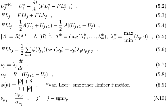
J > 1
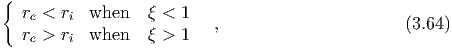
- The particle is initially at the periastron of its elliptical orbit. There is
a value Je such that if J > Je the particle escapes to infinity, if J < Je
the particle orbit becomes circular at t = ∞, and of radius re bigger than
ri.
-
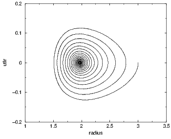
J < 1
- The particle is initially at the apastron of its elliptical orbit. The particle
orbit becomes circular at t = ∞, and of radius re smaller than ri. If
J ≪ 1 the shell relaxation will be fast (it will reach re in a small number
of oscillations) and the quasistatic approximation that we are now going
to describe will break down.
When the timescale of orbital decay by radiation is much longer than the orbital
period, the particle can be considered to be in “quasiequilibrium”. When this condition is
satisfied we are allowed to drop the Φ,tt (radiative) term from the field equation. Doing
this the problem reduces to the solution of three ordinary differential equations which can
be solved “analytically”. We will call this simpler problem the “static” approximation to
the exact problem,
In the static approximation (which reduces to Newtonian gravity in the limit α ≫ 1) the
particle motion is conservative but not necessarily periodic due to the nonlinearity of the
problem.
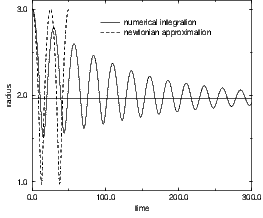
Monitoring the exact solution for the field at a fixed radius rout far from
the particle, one expects a behaviour similar to the one shown in figure 2.3.
In particular the damping of the wave amplitude is due to the fact that the particle is
gradually approaching a circular orbit. In the static approximation the field cannot have
any damping because of the conservativeness of the particle motion, and we get a
behaviour as shown in figure 2.4.
Any reasonable approximation to the exact solution in the nonlinear regime has to be
able to reproduce the damping of the wave. The “quasistatic” approximation that
we propose takes into account the wave damping through the following four
steps:
-
(1)
- We use the solution rp(t) to the static approximation to determine the field equation
source term. We then solve the full field equation, to find the flux of field energy (~ r2Φ
,tΦ,r) radiated out by the gravity wave. This
will allow us to determine the rate of change of the total energy E of the
particle-field system, with respect to time,
-
(2)
- Consider the particle-field system in the stationary state where the particle is
in a circular orbit at a radius R. Then instantaneously change the particle
angular momentum from J = 1 to J = ũϕ∕(ũϕ)circ(R) and calculate the total
energy of the system. Repeating this for all radii R between ri and re we get
a curve E(R) similar to the one shown in figure 2.5. The values E(re) and
E(ri) are exact, while at the true inversion points rinv of the particle orbit,
E(rinv) are expected to be good approximations to the corresponding exact
values. Knowing E(R) we can find the rate of change of E with respect to R.
-
(3)
- Use the chain rule to get the rate of change of R with respect to time,
-
(4)
- Finally knowing dR∕dt we can correct the previous static estimate of the field
equation source term. We can then solve the full field equation again to get the wave
damping.
Chapter 3
Statement of the problem
3.1 Basic Equations
The gravitational field is described by a massless scalar field Φ(xα) in special relativity.
The scalar field does not modify the background space-time geometry which is always
Minkowskian. Consider a particle of rest mass m moving along a world-line zα(λ). Then
the action for the field-particle system is,
where the lagrangian density  is, and where the comoving density is, Here the metric tensor gαβ is the usual Minkowski metric ηαβ since space-time is flat in
this theory [i.e. gαβ = ηαβ = diag(-1, 1, 1, 1) in Cartesian coordinates]. We use arrows to
denote four-vectors and boldface to denote three-vectors. We will set the speed of light
c = 1 but will display the gravitational coupling constant (Newton’ s constant) G
explicitly. If we choose λ equal to the proper time τ along the particle world-line, then,
where γ ≡ dz0∕dτ is the Lorentz factor.
is, and where the comoving density is, Here the metric tensor gαβ is the usual Minkowski metric ηαβ since space-time is flat in
this theory [i.e. gαβ = ηαβ = diag(-1, 1, 1, 1) in Cartesian coordinates]. We use arrows to
denote four-vectors and boldface to denote three-vectors. We will set the speed of light
c = 1 but will display the gravitational coupling constant (Newton’ s constant) G
explicitly. If we choose λ equal to the proper time τ along the particle world-line, then,
where γ ≡ dz0∕dτ is the Lorentz factor.
Varying the Lagrangian (3.2) with respect to Φ gives the field equation of motion,
In the Newtonian limit, where Φ ≪ 1, equation (3.6) becomes linear and reduces to
Poisson’ s equation. Varying the lagrangian with respect to zα gives the particle equation
of motion, where D denotes covariant differentiation. Here we are allowing for curvilinear
coordinates; covariant differentiation reduces to ordinary differentiation in Cartesian
coordinates. In the non relativistic limit equation (3.7) implies that the gravitational force
is -∇Φ. The fully relativistic form ensures that the four-velocity uα = dzα∕dτ remains
orthogonal to the four-acceleration aα = Duα∕dτ.
3.2 The problem
Consider one particle of rest mass m moving along a world-line zα(τ) = (r
p,t) with
four-velocity uα, under the influence of a massless scalar gravitational field Φ(r,t) in
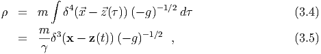
special relativity. In spherical symmetry the comoving matter density takes the form,
where r = |r| and γ = u0 is the Lorentz factor. The particle effectively represents an entire
spherical shell of radius rp and mass surface density σ = m∕(γ4πrp2).
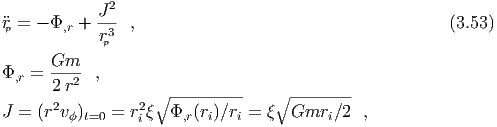
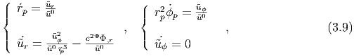
Assuming the particle confined in the θ = π∕2 plane, so that uθ = 0 at all
times, the equations of motion in spherical coordinates rp = (rp,θp,ϕp), are,
where, and we use the dot to denote total differentiation with respect to time, and commas to
indicate partial differentiation.
The particle moves conserving its orbital angular momentum ũϕ. For a static
gravitational field the particle energy ũ0 is also a constant.
Notice that from the field equation (3.6) follows that ϕ,r has, at all times
, a
jump of 4πGeΦσ at the shell surface r = r
p(t). It is then necessary to specify how we
calculate the gravitational force felt by the shell. We will use in equation (3.9),
In this way we prevent any small patch of surface on the shell from interacting with
itself.
3.3 Initial condition
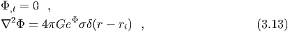
The field starts from a moment of time symmetry, so that at t = 0,
where ri = rp(t = 0) is the initial shell radius. The field is subject to the boundary
conditions, Choosing, we can determine ai = a(t = 0) from the matching condition at the shell’ s surface,
Initially the particle is in a circular orbit of radius ri around the origin, with an angular momentum, We can then find ai from equation (3.17), which becomes,
This initial condition (an Einstein state) is a stationary wave for the field equation of
motion and a stable circular orbit for the particle. So if we let the system evolve from this
initial state nothing will happen: the particle will keep moving in the circular orbit at
radius rp(t) = ri under the influence of the static gravitational field (3.16). This can be
shown, for example, rewriting the field equation of motion in terms of the auxiliary
functions,
Now equation (3.6) becomes, where F = Gm exp(2Φ)∕(2rpũ0). The initial condition for X and Y becomes,
From equations (3.19) and (3.20) follows that when ξ = 1, at t = 0, the source term
F = ai∕(2ri). So that after an infinitesimal timestep dt, X(r,dt) = X(r, 0) and
Y (r,dt) = Y (r, 0).
So we perturb the system changing the particle’ s angular momentum by a factor ξ,
and let it evolve.
3.4 Conserved integrals
The particle-field dynamical system is characterized by a time-varying matter and
velocity profile, interacting with a time varying scalar field containing radiation.
Conservation of energy-momentum follows from,
where T is the total stress-energy tensor of the system, Carrying out the variation using equation (3.2) we find, where,
Conservation of energy-momentum gives rise to the following conserved integrals,
where Sr is the volume of the sphere of radius r centered at the origin, and we used
spherical symmetry in the last equality.
When r > rp(t) we find,
The particle-field total mass energy is given by the integral in equation (3.31),
According to equation (3.31), when evaluated at large enough radius, outside any
radiation or matter, E is conserved. As the particle shell breaths around its asymptotic
virial equilibrium state, Eparticle will undergo exponentially dumped oscillations around its
asymptotic value (see figure 3.1): the oscillations are due to the coupling with the field,
and the dumping to the gravitational radiation going out to infinity (as a gravity wave).
So that after a long time, apart from some particular combinations of ξ and ri∕m (see
section 3.6.2), some energy will have been exchanged between the field and the particle.
For a static situation, the (Φ,r)2 term in equation (3.32) can be integrated by parts to
get,
where Φp = Φ(rp,t). In the Newtonian limit equation (3.33) becomes, where vi ≡ ui∕u0. So E is the sum of the rest mass, plus the kinetic energy, plus the
gravitational potential energy of the matter shell.
When r < rp(t),
which implies,
Those conserved integrals can be used as self consistent checks on our numerical
integration. In figure 3.2 we show what we would expect if we were to evaluate the energy
conservation equation,
as a function of time at two fixed radii rec. The first radius is inside the shell at all times,
the second is always in the vacuum exterior. In the first case the right hand side of
equation (3.39) is zero, the integrated flux term (second integral in equation (3.39)) is
large, and the energy conservation involves the cancellation of large terms. Consequently,
the high degree to which we are able to maintain energy conservation is a nontrivial
measure of the accuracy of the code. In the exterior, the flux is small and energy
conservation is not a stringent test.
3.5 Monopole radiation
In the weak field, slow motion limit, the radiation field can be obtained by a multipole
expansion. Since the theory involves a scalar field, the lowest-order contribution to the
radiation comes from the monopole term. This is in contrast with electromagnetism
(vector field: dipole radiation) or general relativity (tensor field: quadrupole
radiation).
Using Green’ s function for the wave equation we can transform equation (3.6) into
the integral form,
In the wave zone we can replace the denominator in equation (3.40) by the distance
r = |x|. To isolate the conserved rest mass m, define the rest density to be,
Then, In the integrand, expand, and, where v2 = [u
r∕u0]2 + [u
ϕ∕(u0r)]2. For large r, The leading-order contribution to the expansion of equation (3.42) comes from the
product of ρ0 in equation (3.43) with the 1 in equation (3.44). The resulting integral gives
m, so that this term represents the nonradiative Coulomb field. Thus the leading-order
radiation field is, To this order, it is irrelevant wether one uses ρ or ρ0 in equation (3.46).
For a spherically symmetric density distribution, the term proportional to cos θ′ in
equation (3.46) integrates to zero, giving,
The last term in the integrand can be rewritten as follows, and using the equation of motion (3.9) in the weak field limit, we find, Thus equation (3.47) becomes, In figure 3.3 we show how a snapshot of the field at t = to should look like, and compare
it with the leading order radiation field of equation (3.50), in the wave zone.
From equation (3.31) follows that the rate of energy emission when r > rp(t) is,
where in the last equality we used the fact that since X is propagating to the left, the
following outgoing wave boundary condition must hold,
3.6 Analytic results
3.6.1 Newtonian limit
For weak fields and slow velocities we can test our code using the analytic solution
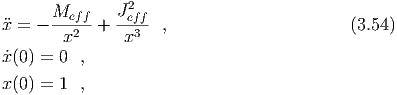
from Newtonian gravitation. In this limit the particle equation of motion is,
which can be rewritten as, where rp(t) = rix(t), Meff = Gm∕(2ri3), and J
eff = ξ . The first integral yields the
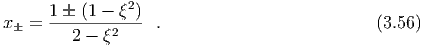
conserved energy, For E = Meff(ξ2∕2 - 1) < 0 (i.e. ξ2 < 2) we have bound orbits. Solving for the turning
points (ẋ = 0) yields, So that for 0 < ξ < 1 the shell contracts to rix- and for 1 < ξ <
. The first integral yields the
conserved energy, For E = Meff(ξ2∕2 - 1) < 0 (i.e. ξ2 < 2) we have bound orbits. Solving for the turning
points (ẋ = 0) yields, So that for 0 < ξ < 1 the shell contracts to rix- and for 1 < ξ <  it expands to rix-.
For ξ >
it expands to rix-.
For ξ >  the shell explodes.
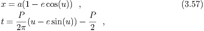
Integrating the equation of motion we get the parametric solution,
where the semimajor axis, eccentricity and period are given by,
Inserting this analytic solution into equation (3.47) and differentiating with respect to
time gives the wave amplitude in the wave zone,
From equation (3.51) we get for the rate of energy emission, Integrating over an oscillation period we get the energy radiated per period,
3.6.2 Relaxation to virial equilibrium
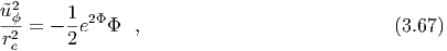
If the shell does not explode or collapse, it will eventually reach, as it loses energy by
emitting gravitational waves, an equilibrium circular orbit (see figure 3.4). At this point
the particle-field system is in an Einstein state were ũr = 0, ũϕ2 = r
p3e2ΦΦ
,r,
and the field is static and of the form (3.16), in a neighborhood of the shell.
Given the angular momentum of the particle ũϕ we can then predict the final
equilibrium radius re, by solving the following equations in ae = a(t = ∞) and
re = rp(t = ∞),
One can verify that,
This final state is a virial equilibrium state. Taking the trace of the special relativistic
virial theorem,
gives at equilibrium, or, when ũr = 0, which is the same as equation (3.63), when the field is of the form (3.16).
The final energy of the particle-field system is,
where,
The shell will only collapse into the origin when it possesses 0 angular momentum
. This
follows from equation (3.10) and the observation that the particle energy mũ0 will always
be smaller than the initial total energy of the particle-field system E(t = 0). Since the
exponential is bigger than 0, we can write,
and when ũr = 0, equation (3.70) gives the following lower bound on the accessible radii
,
where,
3.6.3 Explosion
In order to explode the shell has to reach r = ∞ with at least ũr = 0. But for r →∞,
σ → 0 and ϕ → 0 so that Eparticle → m. When the shell is at infinity Efield will be a small
positive quantity. So for the explosion to happen the initial energy of the particle-field
system has to be greater then m,
In the Newtonian limit ri ≫ m, condition (3.73) reduces to ξ >  . The escape radial
velocity is (see figure 3.5), or,
. The escape radial
velocity is (see figure 3.5), or,
Chapter 4
Approximations
Here we will describe two approximated solutions of the exact problem stated in chapter
3.
4.1 Quasistatic approximation
When it takes many oscillations for the particle to settle into the final stable circular
orbit, we can hope to approximate its slow motion with a quasistatic approximation. The
idea is the following. Consider the static version of our problem (equations (3.9)-(3.6)),
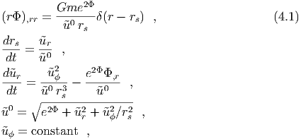
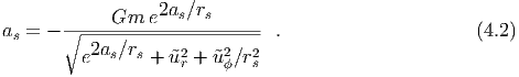
where we called rs(t) the shell radius in this static approximation. At all times the field
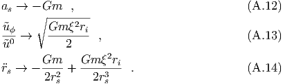
must be of the form (3.16) with a = as. Once we know rs(t) and ũr(t) we can determine
the field from the jump condition (3.17), Since we have a static field Φ = Φ(r,rs(t),ũr(t)), Φ,t = 0 and the system is
conservative. The shell will then experience undumped oscillations around its final
equilibrium radius re. In order to have the shell reach re, we need a recipe to dump
the oscillations. This will give us a quasistatic approximation to the true shell
motion.
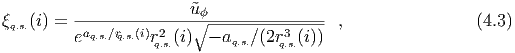
Once we know the initial ri, and final re shell radii we can construct a sequence of
intermediate “quasi-static” Einstein states as follows. The shell initially at ri will contract
(ξ < 1) or expand (ξ > 1) towards re in a succession of circular orbits (ũr = 0) occurring
at the true inversion points of the particle trajectory. We call the intermediate radii of
these circular orbits, rq.s.(i) = rp(P1 + … + Pi), where P1,…,Pi are the first i oscillation
periods . At those points the field will be of the form (3.16) with a = aq.s. determined by
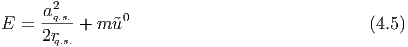
solving equation (3.17) for any given rp = rq.s.(i). At each rq.s. we can determine the new
value of ξ,
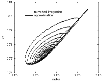
the particle energy, and the particle-field energy, We expect this to be a very good approximation for the particle energy at the true
inversion points of the particle trajectory for a wide range of α’s and ξ’s (see figures 4.1
and 4.2).
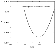
There usually is a value of ξ different from 1, ξo, at which the energy of the particle in
the final equilibrium state is equal to its energy at the beginning of the evolution (see
figure 4.3). For shells with α < 0.4204623..., ξo < 1, for less compact shells ξo > 1.
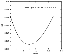
One can also show that E(rq.s.) has a minimum at rq.s.(∞) = re (see figure 4.4).
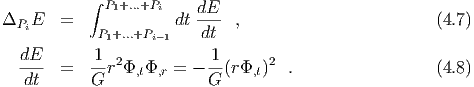
Suppose we have approximated the true shell motion up to the i-th period Pi. Then
we continue the approximation as follows (see figure 4.5),
-
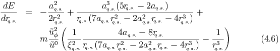
1.
- Calculate dE∕drq.s. from equation (4.5),
-
2.
- Calculate the energy radiated in the i-th oscillation period Pi. In general, when
r > rp(t), We need a good approximation to the monopole term (the lowest order contribution
to the radiation) of the wave amplitude rΦ(r,t). In the weak field slow motion limit
one finds (see equation (3.47)), When α ≫ 1 it will be sufficient to use the Newtonian approximation. So we will
use the analytic expression (3.61). When α ~ 1 we need to use the static
approximation (system (4.1)) to get a numerical estimate for ΔPiE. The details of
the calculation are outlined in the appendix.
-
3.
- Given rq.s.(i) we can find rq.s.(i + 1) using the chain rule,
-
4.
- Start a new static oscillation from ri = rq.s.(i + 1) and ξ = ξq.s.(i + 1).
4.2 Characteristics approximation
We adopt a mean-field particle simulation scheme:
-
1.
- The particle is evolved in the mean background field Φ for a small time Δt.
-
2.
- From the new particle position and velocity we obtain the new matter source
term appearing in the field equation (3.6).
-
3.
- We then update Φ by evolving the field equation for a time-step Δt.
-
4.
- Repeat the whole process.
The particle evolves through an ordinary differential equation which poses no computational
difficulties. One can for example use one of the standard Runge-Kutta schemes to solve it.
The field evolution is much more problematic. It involves the solution of the
Cauchy problem for a non-linear hyperbolic partial differential equation with
discontinuous initial data. In the next chapter we will outline an exact numerical
integration scheme for the field equation. Here we will describe an approximated
one.
The idea is to use the auxiliary functions X(r,t) and Y (r,t) introduced in section 3.3.
We make the following approximation: in the timestep dt we evolve the field according
to equation (3.22) where we consider the source term F as constant in time
.
Under this approximation, given at time to, X(r,to) = Xo(r), and Y (r,to) = Y o(r) the
solutions for X and Y at later times are,
where st[a,b](r) = H(x - a) - H(x - b) with H the Heaviside
function, Δt = t - to, and we added an image soruce at r = -rp(t)
in
order to ensure the finiteness of the field at the origin at all times, which requires,
We then reconstruct the gravitational field as follows,
In our code we tabulate the field using a uniform grid in r and we choose dr = dt. We
need infact, to make sure that in using the solutions (4.10), the source terms fall upon the
translated functions less frequently as possible. Those events are purely due to the
mean field scheme, which require that we move the particle over a fixed field.
When dr = dt they occur only when the particle hits a grid point at a given
timestep.
Chapter 5
Exact Numerical Integration
Here we describe the scheme we use to solve exactly the scalar field equation (3.6) coupled
to the particle equations (3.9) in spherical symmetry, within the mean-field approximation
described in secction 4.2.
5.1 Characteristics method
In order to make to make the characteristics approximation an exact integration we need
to replace the solution (4.10) with,
In our numerical integration we have always used the field time-step Δt, equal to
the particle time-step dt, equal to the grid spacing dr. In this case there is no
difference in using equations (5.1) or (4.10). If we want to use Δt = ndt with
n = 2, 3,… then the more general solution (5.1) should be used and solved by
iteration.
5.2 High resolution method
A more rigorous method when computing discontinuous solutions of the wave equation
can be found among the flux-limiter methods described in chapter 16 of Randall J.
LeVeque “Numerical Methods for Conservation Laws”. Here we will describe the one
employing the “Van Leer” smoother limiter function.
This method is second order accurate on smooth parts of the field and yet gives a well
resolved, nonoscillatory discontinuity at the shell surface (by increasing the amount of
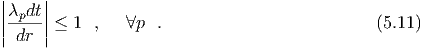
numerical dissipation in its neighborhood). The method has the total variation
diminishing property provided that the Courant, Friedrichs, and Lewy (CFL) condition is
satisfied and consequently it is mononotonicity preserving.
We will first state the method for a general linear hyperbolic system of partial
differential equations and later specialize it to our nonlinear field equation.
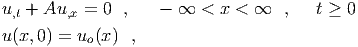
Consider the time-dependent Cauchy problem in one space dimension,
where u ∈ Rm and A is an n × n matrix. The system is called hyperbolic when A is
diagonalizable with real eigenvalues, so that we can decompose A = RΛR-1, where
Λ = diag(λ1,λ2…,λm) is the diagonal matrix of eigenvalues and R = [r1|r2| |rm] is the
matrix of right eigenvectors of A. Discretize time as tn = ndt and space as xj = jdr. The
finite difference method we want to describe produces approximations Ujn ∈ Rm to the
solution u(xj,tn) = ujn at the discrete grid points. The method is written in conservative
form as follows, FLh is the high order (Lax-Wendroff) flux acting on the smooth portions of the solution
(where θ is near to 1) while FLl is the low order (first order upwind) flux acting in
the vicinity of a discontinuity (where θ is far from 1). The CFL condition is,
|rm] is the
matrix of right eigenvectors of A. Discretize time as tn = ndt and space as xj = jdr. The
finite difference method we want to describe produces approximations Ujn ∈ Rm to the
solution u(xj,tn) = ujn at the discrete grid points. The method is written in conservative
form as follows, FLh is the high order (Lax-Wendroff) flux acting on the smooth portions of the solution
(where θ is near to 1) while FLl is the low order (first order upwind) flux acting in
the vicinity of a discontinuity (where θ is far from 1). The CFL condition is,
Our field equation is a wave equation with a nonlinear source term. It can be rewritten
as follows,
The initial condition is, If we call rmax = jmaxdr the maximum extent of our grid, the outgoing wave boudary
conditions are, Immagine that we have approximated the true solution of the field equation up to the
n-th time slice (i.e. we know Ujn for j = -j
max,…,-1, 0, 1,…,jmax). The difference
scheme, when evaluated at jmax becomes a system of 2 equations in 2 unknowns U1jmaxn+1 and
U1jmax+1n, allowing the closure of the difference scheme. A consistency check would be to monitor
the constraint,
The difference scheme to be used for the field equation follows from equation (5.2),
where B is the approximation to the source term b, In equation (5.26) we have approximated the delta functions using a triangular
shaped cloud scheme, which in one dimension employs 3 mesh points and has
an assignment-interpolation function W which is continuous in value and first
derivative. Mass is assigned from the particle at rp to the 3 mesh points nearest to it,
Chapter 6
Numerical results
When analyzing our numerical results, we will adopt gravitational units where G = c = 1.
In this chapter we report the results obtained with the characteristic approximation
code (see section D). We will refer to this results as the “exact integration”
results.
6.1 Relaxation to virial equilibrium
When trying to reproduce the expected behaviour described in figure 3.4 we got figure
6.1.
When trying to reproduce the expected behaviour described in figure 3.1 we got figure
6.2.
6.2 C omparison with the analytic method
We compare the numerical integration in the linear and nonlinear regimes with the
analytic Newtonian solution.
6.3 Monopole radiation
When trying to reproduce the expected behaviour described in figure 3.3 we got figure
6.6.
6.4 Quasistatic approximation
When trying to reproduce the expected behaviour described in figure 4.1 we got figures
6.7 and 6.8.
Chapter 7
Conclusions
Some future developments to the present work may be:
-
0
- Correct the characteristics approximation as outlined in section refcharacteristics
-
1
- Integrate the equations (3.6) and (3.7) using the finite-difference scheme for the
evolution of the field described in section 5.2.
-
2
- Extend the one particle problem to a many particle one, and check how the
quasistatic approximation performs there.
-
3
- Go on to solve more realistic gravitational field theories, and look for quasistatic
approximations.
Appendix A
Energy loss in the static approximation
In the weak field slow motion limit, in the wave zone the gravity wave amplitude can be
written (dropping terms higher than the monopole) as (see equation (3.47) in the main
text),
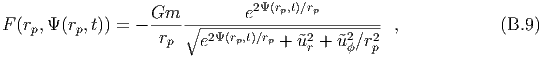
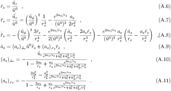
where in the static approximation, and as = as(rs,ũr) through the jump condition (see equation (4.2) in the main text),
Then we can rewrite the wave amplitude as follows, Taking the time derivative one gets (both ũ0 and ũ
ϕ are constants of motion),
In the static approximation,
Using equations (A.6)-(A.11) into equation (A.5) one can determine numerically the
rate of energy loss (3.51). This can then be integrated to get the energy emitted by the
particle in a full revolution around the origin. This calculation can be carried out
analytically in the Newtonian approximation as shown in detail in the next
section.
A.1 Newtonian approximation
In the Newtonian approximation we have,
Making these substitutions in equation (A.5) we get equation (3.59) of the main text,
where x = rs∕ri. So for the rate of energy emission in the wave zone we get equation
(3.60), which integrated over one orbital period gives equation (3.61).
Appendix B
Method of Images
We want to justify the use we have made of the images method, in the solution of the
nonlinear field equation (3.6).
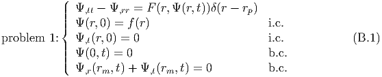
To do that we need to show the equivalence between the two following problems.
Calling Ψ(r,t) = rΦ(r,t), with r ∈ [0,∞], the first problem is our original one, namely,
where i.c. stands for initial condition and b.c. for boundary condition.
The second problem is over the whole real axis x ∈ [-∞,∞] and employs two sources,
the one at rp, of the first problem, and its image,
The general solution to problem 1 can be written in integral form as follows,
where, and the last term in equation (B.3) was added in order to have the solution satisfy the
boundary condition at r = 0. The outgoing wave boundary condition is automatically
satisfayed since rm is intended to be at all times to the right of the source, and
f(r) is constant for r > rp(0). So there are no ingoing waves passing through
rm.
The general solution to problem 2 can be written in integral form as follows,
In order for the two problems to have the same solution for x ≥ 0, the following
condition has to be satisfied,
This condition is equivalent to, where in the last equality we used the fact that the field is an odd function in x at all
times. We can easily verify that our field equation, where, satisfies such condition.
Appendix C
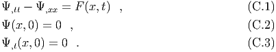
The nonhomogeneous wave equation
We want to find a solution to the following problem,
Make the change of variables, The differential equation then becomes, Integrating with respect to ξ, we have, We integrate this equation from an arbitrary value of η to ξ to find, In the first integral we note that, In the second integral we let, The domain of integration η ≤η ≤ξ ≤ ξ becomes or The jacobian determinant of the transformation from (ξ,η) to (x,t) is 2. Therefore
Making these substitutions and transposing, we find We recall that ξ = x + t and η = x-t. We use the initial conditions to obtain the solution
formula
Appendix D
The code
This is the code
used for the exact numerical integration.
ccccccccccccccccccccccccccccccccccccccccccccccccccccccccccccccc
c 1 SHELL CLUSTER
c dimt = number of timesteps in the integration
c dimg = dimension of the uniform r grid
c
c INPUT r0=shell radius
c mr=shell rest mass
c xi=up/up(circular)
c dt=time-step
c rot=dr/dt dr=grid spacing
c OUTPUT
c fort.8 = (t,rp)
c fort.9 = (rp,utt,utlr)
c erp=equilibrium radius
ccccccccccccccccccccccccccccccccccccccccccccccccccccccccccccccc
implicit none
include ’cluster.p’
c INPUT
real*8 r0,mr,xi
real*8 dt
integer rot
c OUTPUT
real*8 erp,rp,utt,utlr
c INTERNAL
real*8 phirp,e2p,fpl,fpr,phiprp,e2ppr,st
real*8 a,ea,dr
real*8 ut,up,utlp,am2
real*8 xx(0:imax),yy(-imax:imax)
real*8 rg(-imax:imax),phi(0:imax)
integer i,tsteps,jp,dimg,dimt
parameter(dimg=1000)
parameter(dimt=60000)
c ========================INPUT DATA============================
call in(rp,mr,xi,dr,rot,dt)
r0=rp
c =====================INITIAL CONDITION========================
tsteps=0
c -------------uniform grid in r (spacing dr)-------------------
do i=-dimg,dimg
rg(i)=dble(i)*dr
enddo
c ----------particle--------------------------------------------
c tangential orbit (utlr=0)
utlr=0.d0
c find angular velocity for the circular orbit at rp
call phi1(mr,rp,a,up)
c angular momentum for circular orbits (in a time
c independent field) is:
c utlp(circ)=ulp(circ)*exp(phi)=up(circ)*r*r*exp(phi)
c set utlp=xi*utlp(circ) = constant of motion
utlp=xi*rp**2*exp(a/rp)*up
am2 =utlp**2
up=utlp/(rp**2*exp(a/rp))
ut=sqrt(1.d0+(rp*up)**2)
c initial source term
st=exp(a/rp)*mr/(2.d0*rp*ut)
c ----------field-----------------------------------------------
c xx(r,0)=yy(r,0)=(r*phi(r,0)),r
c phi(r,0)=a/rp r <= rp
c phi(r,0)=a/r r > rp
jp=nint(rp/dr)
c real space r >= 0
do i=0,jp-1
xx(i)=.5d0*a/rp
yy(i)=.5d0*a/rp
phi(i)=a/rp
enddo
do i=jp,dimg
xx(i)=0.d0
yy(i)=0.d0
phi(i)=a/rg(i)
enddo
c immaginary space r < 0
do i=-dimg,-jp-1
yy(i)=0.d0
enddo
do i=-jp,-1
yy(i)=.5d0*a/rp
enddo
c =====================NEXT TIMESTEP============================
100 tsteps=tsteps+1
if(mod(tsteps,rot).ne.0) goto 15
c ----------evolve field----------------------------------------
c reinterpolate phi(rp) to find new source term
jp =nint(rp/dr)
phirp=phi(jp)
e2p = exp(2.d0*phirp)
utt = sqrt(e2p+utlr**2+(utlp/rp)**2)
c the new source term is
st = .5d0*e2p*mr/(rp*utt)
c evolve the field
call evphi(dimg,dr,rg,st,rp,xx,yy,phi)
c ----------evolve particle-------------------------------------
c find e2p=exp(2*phi(rp))
15 jp = nint(rp/dr)
phirp = phi(jp)
e2p = exp(2.d0*phirp)
c find e2ppr=e2p*(phi,r(rp-)+phi,r(rp+))/2
fpl = (xx(jp-1)+yy(jp-1)-phirp)/rp
fpr = (xx(jp+1)+yy(jp+1)-phirp)/rp
phiprp= (fpl+fpr)*.5d0
e2ppr = e2p*phiprp
c evolve the particle with 4-th order Runge-Kutta
call runge4(am2,e2p,e2ppr,dt,rp,utlr,rp,utlr)
c write fort.8 :[t,r(t)] and fort.9 :[t,utt(t),utlr(t)]
write(8,*) tsteps*dt,rp,phirp
write(9,*) rp,utt,utlr
if(tsteps.eq.dimt) goto 200
goto 100
c estimate the final equilibrium radius erp
200 call eqrp1(utlp,mr,erp,ea)
c write output
call out(mr,r0,erp,xi,dt,dr,dimt,dimg)
stop
end
cccccccccccccccccccccccccccccccccccccccccccccccccccccccccccccc
c Read initial data
c INPUT
c rp = initial shell radius
c mr = shell rest mass
c xi = ratio up/up(circular)
c dt = time-step
c rot = dr/dt(>=1 Courant stability condition)
c
c OUTPUT(all above +)
c dr = grid spacing
cccccccccccccccccccccccccccccccccccccccccccccccccccccccccccccccc
subroutine in(rp,mr,xi,dr,rot,dt)
implicit none
real*8 rp,mr,xi,dr,dt
integer rot
write(*,*) ’initial radius rp’
read(*,*) rp
write(*,*) ’rest mass mr’
read(*,*) mr
write(*,*) ’ratio utlp/utlp(circular)’
read(*,*) xi
write(*,*) ’time-step dt’
read(*,*) dt
write(*,*) ’ratio dr/dt=[integer>=1]’
read(*,*) rot
dr=dt*dble(rot)
return
end
cccccccccccccccccccccccccccccccccccccccccccccccccccccc
c 4-th order runge-kutta
c advances to the next time step (h) the equations
c dr/dt=f(r,u)
c du/dt=g(r.u)
c where u=utlr (u tilde-low-r)
c f(r,u)=u/utu0
c g(r,u)=utlp**2/(utu0*r**3)-exp(2*phi)*phi,r/utu0
c utu0=sqrt(exp(2*phi)+u**2+(utlp/r)**2)
c and phi = potential at r,u
c phi,r = d(phi)/dr at r,u
c INPUT am2(=utlp**2 angular momentum squared),
c e2p(=exp(2*phi)),e2ppr(=exp(2*phi)*phi,r),
c h(=time step),ri,ui(=initial values for r,u)
c OUTPUT r,u (=final values for r,u)
cccccccccccccccccccccccccccccccccccccccccccccccccccccc
subroutine runge4(am2,e2p,e2ppr,h,ri,ui,r,u)
implicit none
c INPUT
real*8 am2,e2p,e2ppr,h,ri,ui
c OUTPUT
real*8 u,r
c INTERNAL
real*8 f,g,u0
real*8 k1,k2,k3,k4,l1,l2,l3,l4
real*8 k1o2,k2o2,l1o2,l2o2
real*8 inv6
parameter(inv6=1/6.d0)
u0(r,u)= sqrt(e2p+u**2+am2/r**2)
f(r,u) = u/u0(r,u)
g(r,u) = am2/(u0(r,u)*r**3)-e2ppr/u0(r,u)
k1 = h*f(ri,ui)
l1 = h*g(ri,ui)
k1o2= .5d0*k1
l1o2= .5d0*l1
k2 = h*f(ri+k1o2,ui+l1o2)
l2 = h*g(ri+k1o2,ui+l1o2)
k2o2= .5d0*k2
l2o2= .5d0*l2
k3 = h*f(ri+k2o2,ui+l2o2)
l3 = h*g(ri+k2o2,ui+l2o2)
k4 = h*f(ri+k3,ui+l3)
l4 = h*g(ri+k3,ui+l3)
r = ri+inv6*(k1+2.d0*(k2+k3)+k4)
u = ui+inv6*(l1+2.d0*(l2+l3)+l4)
return
end
cccccccccccccccccccccccccccccccccccccccccccccccccccccccccccc
c Integrate the 1D wave equation with a delta
c function as the source
c -(r*phi),tt+(r*phi),rr=2*st*delta(r-rp)
c rewritten as
c xx,t=xx,r+st*delta(r-rp)
c yy,t=-yy,r-st*delta(r-rp)
c where
c xx=(v+w)/2
c yy=(v-w)/2
c and
c v=(r*phi),r
c w=(r*phi),t
c add an image to ensure finiteness of phi(0,t) forall t
c xx(0,t)=yy(0,t) at all times
c
c INPUT dr (= grid spacing), rg(-imax:imax) (= grid),
c st (= source term), rp (= shell radius),
c xxo(0:imax), yyo(-imax:imax) (= old "field")
c
c OUTPUT xxo(0:imax), yyo(-imax:imax), phi(0:imax) (=field)
cccccccccccccccccccccccccccccccccccccccccccccccccccccccccccc
subroutine evphi(dimg,dr,rg,st,rp,xxo,yyo,phi)
implicit none
include ’cluster.p’
c INPUT
integer dimg
real*8 st,dr,rp
real*8 rg(-imax:imax)
c OUTPUT
real*8 xxo(0:imax),yyo(-imax:imax)
real*8 phi(0:imax)
c INTERNAL
real*8 xx(0:imax),yy(-imax:imax)
real*8 dt,psi
integer i
c check for rp>=rg(dimg-1)
if(rp.ge.rg(dimg-1)) then
write(*,*) ’particle out of right grid margin !!!’
stop
endif
c field timestep
dt=dr
c yy(r)=yyo(r-dt)+st*step[rp,rp+dt]-st*step[-rp,-rp+dt]
c xx(r)=xxo(r+dt)-st*step[rp-dt,rp]
yy(-dimg)=0.d0
do i=-dimg+1,-1
yy(i)=yyo(i-1)
if(-rp.le.rg(i).and.rg(i).lt.-rp+dt) then
yy(i)=yy(i)-st
endif
enddo
do i=0,dimg-1
xx(i)=xxo(i+1)
yy(i)=yyo(i-1)
if(rp-dt.le.rg(i).and.rg(i).lt.rp) then
xx(i)=xx(i)-st
elseif(rp.le.rg(i).and.rg(i).lt.rp+dt) then
yy(i)=yy(i)+st
endif
enddo
xx(dimg)=0.d0
yy(dimg)=yyo(dimg-1)
c rewrite xx and yy
do i=-dimg,-1
yyo(i)=yy(i)
enddo
do i=0,dimg
xxo(i)=xx(i)
yyo(i)=yy(i)
enddo
c integrate x+y starting from the origin
c using trapezoidal method (order dr**3)
psi=.5d0*(xx(0)+yy(0))
do i=1,dimg
psi=psi+xx(i)+yy(i)
c the gravitational potential is
phi(i)=dr*(psi-.5d0*(xx(i)+yy(i)))/rg(i)
enddo
phi(0)=phi(1)
c check boundary condition at r=0
if(xx(0).ne.yy(0)) then
print *,’xx(0) <> yy(0) !!!!!!!!’
endif
return
end
cccccccccccccccccccccccccccccccccccccccccccccccccccccccccccc
c Given rp (and ur=0) solves for a and up in:
c 1.0) ut = sqrt(1+ur**2+(rp*up)**2)
c 1.1) a =-exp(a/rp)*mr/ut
c 2 ) up = sqrt(-a/(2*rp**3))
c rewritten as
c -a = exp(a/rp)*mr/sqrt(1-a/(2*rp))
c
c INPUT mr (= rest mass),rp (= shell radius)
c OUTPUT a ("potential"), up (= angular velocity)
cccccccccccccccccccccccccccccccccccccccccccccccccccccccccccc
subroutine phi1(mr,rp,a,up)
implicit none
c INPUT
real*8 mr,rp
c OUTPUT
real*8 a,up
c INTERNAL
real*8 ao,sqti,ep,f,fp
real*8 acc
parameter(acc=1.d-15)
a=0.d0
c start the Newton iteration
10 sqti=1.d0/sqrt(1.d0-a/(2.d0*rp))
ep=exp(a/rp)
f=a+mr*ep*sqti
fp=1.d0+mr*ep*(sqti+.25d0*sqti**3)/rp
ao=a
a=ao-f/fp
if(abs(f).gt.acc) goto 10
c the angular velocity rp*up**2=(a/rp**2)/2
up=sqrt(-a/(2.d0*rp**3))
return
end
cccccccccccccccccccccccccccccccccccccccccccccccccccccccccccc
c Finds the equilibrium radius
c given utlp solves for a and rp in:
c 1.0) utt = sqrt(exp(2*a/rp)+(utlp/rp)**2)
c 1.1) a =-exp(2*a/rp)*mr/utt
c 2) utlp**2=-exp(2*a/rp)*rp**3*(a/rp**2)/2
c rewritten as
c y=4*a**4/(a**4-(2*utlp*mr)**2)
c 1) utlp**2*(y/a**2)=-exp(y) -------> find a (<0)
c 2) r=(a**4-(2*utlp*mr)**2)/(2*a**3) -------> find r (>0)
c INPUT utlp (= angular momentum), mr (= rest mass)
c OUTPUT erp (= equil radius),ea (= equil "potential")
cccccccccccccccccccccccccccccccccccccccccccccccccccccccccccc
subroutine eqrp1(utlp,mr,erp,ea)
implicit none
c INPUT
real*8 mr,utlp
c OUTPUT
real*8 ea,erp
c INTERNAL
real*8 a4,y,ai,af,afo,fi,ff
real*8 acc,u2,fu2m2
parameter(acc=1.d-10)
u2=utlp**2
fu2m2=4.d0*u2*mr**2
c upper limit
ai=0.d0
fi=1
c find the lower limit
af=-sqrt(2.d0*u2*(-1.d0+sqrt(1.d0+(-mr/utlp)**2)))
c start the secant iteration
10 a4=af**4
y =4.d0*a4/(a4-fu2m2)
ff=u2*y/af**2+exp(y)
afo=af
af=afo-ff*(afo-ai)/(ff-fi)
if(abs((af-afo)/afo).gt.acc) then
ai=afo
fi=ff
goto 10
endif
c found a find r
erp=(af**4-fu2m2)/(2.d0*af**3)
ea =af
return
end
cccccccccccccccccccccccccccccccccccccccccccccccccccccccccccccccc
c writes parameters in output
cccccccccccccccccccccccccccccccccccccccccccccccccccccccccccccccc
subroutine out(mr,ri,rf,xi,dt,dr,dimt,dimg)
implicit none
real *8 mr,ri,rf,dt,dr,xi
integer dimt,dimg
c rest mass
write(*,*) ’mr=’,mr
c initial radius
write(*,*) ’ri=’,ri
c xi=up/up(circular)
write(*,*) ’xi=’,xi
c final equilibrium radius
write(*,*) ’rf=’,rf
c time step
write(*,*) ’dtf=’,dt
c grid spacing
write(*,*) ’dr=’,dr
c total integration time=dimt*dtf
write(*,*) ’dimt=’,dimt
c grid dimension r in [0,dimg*dr]
write(*,*) ’dimg=’,dimg
return
end
This is the code used for enveloping the
numerical integration.
ccccccccccccccccccccccccccccccccccccccccccccccccccccccccccccccc
c Relaxation to virial equilibrium
c
c INPUT r0=shell initial radius
c mr=shell rest mass
c xi=up/up(circular)
c
c OUTPUT fort.10 : r_max,utt(r_max),xi
c fort.14 : time,r_max
ccccccccccccccccccccccccccccccccccccccccccccccccccccccccccccccc
implicit none
c INPUT
real*8 r0,mr,xi
c OUTPUT
real*8 utt,r(0:1000),tt
c INTERNAL
real*8 dr,dtdr(0:1000),etot,dedt,dedr
real*8 a,ea,rf,utlp,up,am2
real*8 e2p,npo2pi,xi2
integer i,np
parameter(np=999)
c ========================INPUT DATA============================
write(*,*) ’initial radius r0’
read(*,*) r0
write(*,*) ’rest mass mr’
read(*,*) mr
write(*,*) ’ratio utlp/utlp(circular)’
read(*,*) xi
if(xi.ge.sqrt(2.d0)) then
print *,’qust.f uses Newtonian approx. : xi < sqrt(2)’
stop
endif
c ======================INITIALIZATION==========================
c find angular velocity for the circular orbit at r0
call phi1(mr,r0,a,up)
utlp =xi*r0**2*exp(a/r0)*up
am2 =utlp**2
c find final equilibrium radius rf and particle energy
call eqrp1(utlp,mr,rf,ea)
dr =(rf-r0)/dble(np)
print *,’initial radius, potential=’,r0,a/r0
print *,’final radius, potential=’,rf,ea/rf
print *,’initial energy utt=’,sqrt(exp(2.d0*a/r0) +am2/r0**2)
print *,’final energy utt=’,sqrt(exp(2.d0*ea/rf)+am2/rf**2)
c =================r_{max},xi,utt(r_{max})======================
do i=0,np-1
r(i)=r0+dble(i)*dr
call phi1(mr,r(i),a,up)
e2p=exp(2.d0*a/r(i))
utt=sqrt(e2p+am2/r(i)**2)
c the new xi at r(i) is
xi=utlp/(exp(a/r(i))*up*r(i)**2)
c write fort.10 : (r,utt,xi)
write(10,*) r(i),utt,xi
c the total energy is then
etot=mr*utt
xi2=xi**2
c calculate detot/dr
dedr=(a*r(i)*(4.d0-7.d0*xi2)+a**2*2.d0*xi2+r(i)**2*4.d0
$ *(xi2-2.d0))/(xi2*r(i)**3*(7.d0*a*r(i)-2.d0*a**2-
$ 4.d0*r(i)**2))
dedr=mr*dedr*am2/utt
c calculate detot/dt
npo2pi=sqrt(2.d0*r(i)**3/(a*(xi2-2.d0)**3))
dedt=-(sqrt(2.d0)/9.d0)*mr**2*(sqrt(-a)**5/sqrt(r(i))**7)
$ *((1.d0-xi2)**2/xi**7)*(5.d0-2.d0*xi2+xi**4)/npo2pi
c calculate dr/dt
dtdr(i)=dedr/dedt
enddo
c ====================t,r_max===================================
write(14,*) 0,r0
c integrate (dt/dr) to get t(r)
tt=.5d0*dtdr(1)
do i=1,np-1
tt=tt+dtdr(i)
c make graph (t(r),r)
write(14,*) dr*(tt-.5d0*dtdr(i)),r(i)
enddo
30 stop
end
This is the code used for the quasistatic
integration.
Cccccccccccccccccccccccccccccccccccccccccccccccccccccccccccccccc
c 1 SHELL QUASISTATIC CLUSTER
c
c INPUT rp=shell radius
c mr=shell rest mass
c xi=up/up(circular)
c dt=integration timestep
c time=simulation duration
c OUTPUT
c fort.18 = (t,rp)
c fort.19 = (rp,utt,utlr)
c erp=equilibrium radius
cccccccccccccccccccccccccccccccccccccccccccccccccccccccccccccccc
implicit none
c INPUT
real*8 rp,mr,xi,dt,time
c OUTPUT
real*8 utlr,utt,erp,ea
c INTERNAL
real*8 am2,e2p,e2ppr
real*8 up,a,utlp
integer tsteps,dimt
c ========================INPUT DATA============================
write(*,*) ’initial radius rp’
read(*,*) rp
write(*,*) ’rest mass mr’
read(*,*) mr
write(*,*) ’ratio utlp/utlp(circular)’
read(*,*) xi
write(*,*) ’time step dt’
read(*,*) dt
write(*,*) ’time lenght’
read(*,*) time
dimt=int(time/dt)
c =====================INITIAL CONDITION========================
tsteps=0
c ----------particle------------------------------------
c tangential orbit (utlr=0)
utlr=0.d0
c find angular velocity for the circular orbit at rp
call phi1(mr,rp,a,up)
c angular momentum for circular orbits (in a time
c independent field) is:
c utlp(circ)=ulp(circ)*exp(phi)=up(circ)*r*r*exp(phi)
c set utlp=xi*utlp(circ) = constant of motion
utlp=xi*rp**2*exp(a/rp)*up
am2 =utlp**2
c ----------field---------------------------------------
c phi(r)=a/rp for r<=rp
c phi(r)=a/r for r> rp
c =====================NEXT TIMESTEP============================
100 tsteps= tsteps+1
e2p=exp(2.d0*a/rp)
c find e2ppr=e2p*(phi,r(rp-)+phi,r(rp+))/2
e2ppr=-e2p*.5d0*a/rp**2
c ----------particle-----------------------------------------
c evolve with 4-th order Runge-Kutta
call runge4(am2,e2p,e2ppr,dt,rp,utlr,rp,utlr)
if (rp.le.0.d0) then
print *,’particle fallen in to the origin !!!’
stop
endif
c ----------field--------------------------------------------
call phi1(mr,rp,a,up)
c write fort.18 :[t,r(t)] and fort.19 :[t,utt(t),utlr(t)]
write(18,*) tsteps*dt,rp,a/rp
c calculate utt
utt=sqrt(e2p+utlr**2+am2/rp**2)
write(19,*) rp,utt,utlr
if(tsteps.eq.dimt) goto 200
goto 100
c estimate the final equilibrium radius erp
200 call eqrp1(utlp,mr,erp,ea)
c write erp and the field at erp (ea/erp)
print*,erp,ea/erp
stop
end
Index of figures
2.1 Pictorial evolution of the particle orbit when J > 1.
2.2 Pictorial evolution of the particle orbit when J < 1. 2.3 Expected
behaviour for Φ(rout,t) as a function of time. 2.4 Same as figure 2.3 but in
the static approximation. 2.5 Shows the expected behaviour for the total
energy of the system E as a function of the circular orbits radii R. The energy
curve has its minimum at re, the radius of the circular orbit on which the
particle decays at t = ∞. 3.1 Shows the expected behaviour of the particle
energy ˜ u0 as a function of time for the case α ~ 1 and ξ < 1. 3.2 Energy
conservation at two selected radii as a function of time. The solid line shows
the left-hand side of equation (3.39) (volume integral plus integrated flux),
the dotted line shows the second term alone (integrated flux), and the dashed
line shows the right-hand side (volume integral at t = 0). The radii are (a)
rec < rp(t) at all times, (b)rec > rp(t) at all times. The degree to which the
solid and dashed lines coincide compared with the magnitude of the dotted
line is a measure of the code’ s ability to conserve energy. 3.3 For the case
α ~ 1, ξ < 1, shows a snapshot at t = to of the field Φ(to,r), the first order
radiation part (3.50), and the first order radiation part plus the zeroth order
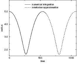
-m∕r. 3.4 Shows the relaxation to the virial equilibrium state for an α ~ 1
shell with two different values of ξ: ξ < 1 and ξ > 1. 3.5 Expected shell
behaviour for ξ > ξe. 4.1 For the α ~ 1, ξ < 1 case, shows ˜ u0 as a function
of the shell radius as expected from an exact numerical integration (solid
line) and from the analytic expression (4.4) (dashed line). We expect the
dashed curve to pass through the true values for the energy at the turning
points of the particle orbit. 4.2 Same as figure 4.1 but for the α ≫ 1 and
ξ < 1 case. 4.3 Shows ˜ u0 as calculated from equation (4.4), as a function
of the shell radius, for two different situations: on the left a more compact
shell, on the right a less compact one. 4.4 Shows the expected family of
curves for E v.s. rp parametrized by the particle’ s angular momentum
ξ. 4.5 How the quasistatic approximation is expected to approximate a
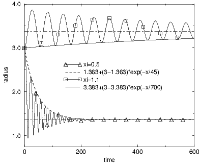
nonlinear collapse. 6.1 Shows the relaxation to the virial equilibrium state
for an α = 3 shell with two different values of ξ. In both cases the decay
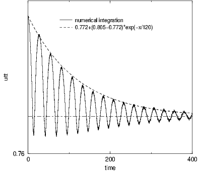
is fitted well by an exponential. 6.2 For the case α = 3, ξ = 0.7 shows the
particle energy ˜ u0 versus time. The decay to the equilibrium value is well
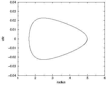
fitted by an exponential. 6.3 Compares the numerical integration with
the analytic Newtonian approximation. To the left the quasi-Newtonian
α = 500, ξ = 0.7 shell is shown. The predicted equilibrium radius is at
re = 2.4662896500. To the right the α = 3, ξ = 0.7 shell is shown. The
predicted equilibrium radius is at re = 1.9657627134. 6.4 Shows ˜ ur as a
function of the shell radius for the case α = 3, ξ = 0.7. 6.5 Same as figure
6.4 for the case α = 500, ξ = 0.7. 6.6 For the case α = 3, ξ = 0.7, shows a
snapshot at t=100 of the field Φ(100,t), the first order radiation part (3.50),
and the first order radiation part plus the zeroth order -m∕r. 6.7 For the
α = 3, ξ = 0.7 case, shows the ˜ u0 as a function of the shell radius for the
numerical integration. The solid line was derived using the analytic expression
(4.4). We see that it approximates well the values for the energy at the
turning points. 6.8 Same as figure 4.1 but for the α = 500, ξ = 0.7 case.
Bibliography
[1] S. L. Shapiro and S. A. Teukolsky, Phys. Rew. D 47, 1529 (1992).


![Φ,r ≡ [Φ,r(rp- ) + Φ,r(rp+)]∕2 . (3.12)](rep14x.png)

![˜ur = 0 ,
ri(u ϕ )2 = [Φ,r(ri- ) + Φ,r(ri+ )]∕2 = - ai-- , (3.18)
circ 2r2i](rep19x.png)
![X (r,t) = [(r Φ),r + (rΦ ),t]∕2 ,
Y (r,t) = [(rΦ ),r - (rΦ ),t]∕2 . (3.21)](rep22x.png)


![2 δ[L (- g)1∕2]
T μν = -------------------- . (3.26)
(- g)1∕2 δgμν](rep27x.png)

![field --1-- 1- ,α
Tμν = 4πG [Φ,μΦ, ν - 2gμνΦ Φ,α] , (3.28)
particle Φ
Tμν = ρe u μuν . (3.29)](rep29x.png)

![[ Φ ( v2 v2 ) ]
E = m - -p-+ ⋅⋅⋅ + (1 + Φp + ⋅⋅⋅) 1 + -r-+ -ϕ2 + ⋅⋅⋅
( 2 ) 2 2r
v2r v2ϕ Φp
≈ m 1 + ---+ --2 + --- , (3.34)
2 2r 2](rep34x.png)
![∂ ∫ r 2 2 2 2
[μ = 0] ∂t- [(Φ,0) + (Φ,r) ]r dr = 2r Φ,0Φ,r , (3.35)
0
[μ = ϕ] 0 =∫ 0 , (3.36)
∂-- r 2 r2 2 2
[μ = r] ∂t 0 Φ,0Φ,rr dr = 2 [(Φ,0) + (Φ,r) ] , (3.37)](rep35x.png)


![∘ --------------field------------2-----
˜ur(r → ∞ ) = ∘ [(E-(t =-0) --E----(t = ∞ ))∕m ] - 1
2
≈ [E (t = 0)∕m ] - 1 , (3.74)](rep75x.png)
![∫
rΦ (r,t) = - G dr ′ 4πr′2[ρ0(Φ - 12v2) + 16rp2ρ0,tt]t-r .](rep86x.png)


![∫
Φ (r,t) = 1- r[X (r,t) + Y (r,t)] dr . (4.12)
r 0](rep90x.png)
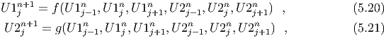
![u,t + Au,x = b , (5.12)
( u1 ) ( Ψ )
u = = ,x , Ψ (x,t) = xΦ (x,t) , (5.13)
( u2 ) Ψ,t ( )
0 - 1 1 0
A = , |A | = , (5.14)
( - 1 0 ) ( 0 1) ( )
- 1 0 1 1 -1 1∕2 1∕2
Λ = 0 1 , R = 1 - 1 , R = 1∕2 - 1∕2 , (5.15)
( )
∫x 0
b = 4πG σe 1x 0 u1(x′,t)dx′x[δ(x - r ) + δ(x + r )] . (5.16)
p p
(5.17)](rep96x.png)

uo(x) = 0 . (5.18)](rep97x.png)


![∫
rΦ (r,t) = - G dr′ 4πr ′2[ρ (Φ - 1v2) + 1r2ρ ] ,
0 2 6p 0,ttt-r](rep113x.png)
![{ a (˙r )2 (˜u )2 1 1 }
rΦ(r,t) = - Gm -s-- --s--- --ϕ ----+ -[(˙rs)2 + rs¨rs] ,
rs 2 u˜0 2r2s 3 t-r
{ a ( ˜u )2 1 1 1 }
= - Gm -s-- -ϕ0- --2-- --(˙rs)2 + --rsr¨s . (A.4)
rs ˜u 2rs 6 3 t- r](rep116x.png)
![4 (Gm )2 [ ˙x ]
rΦ,t = ---------- --2 , (A.15 )
3 ri x t-r](rep120x.png)
![(
||| Ψ,tt - Ψ,xx = F (x,Ψ (x,t))[δ(x - rp) + δ(x + rp)]
{ Ψ (x,0) = f(x) - f(- x) i.c.
problem 2:|| Ψ,t(x,0) = 0 i.c. (B.2)
|( Ψ (±r ,t) ± Ψ (±r ,t) = 0 b.c.
,x m ,t m](rep122x.png)
![∫ t
W (r,t) = dt F (r ,Ψ (r ,t))[H (r - r + (t - t)) - H (- r + r + (t - t))] (B.4)
rp 0 p p p p](rep124x.png)


![( ξ + η ξ - η ) ( ξ + η ξ - η) ]
Ψ, η -----,------ = Ψ η -----,------ (C.7)
2 2 2 2 ξ=η
∫ ξ ( -- -- ) --
+ Ψ,ξη ξ +-η,ξ---η- dξ (C.8)
η 2 2
1 1
= --Ψ,x(η,0) - -Ψ,t(η,0) (C.9)
2∫ ξ (-- 2 -- )
- 1- F ξ-+-η-,ξ --η- dξ- (C.10 )
4 η 2 2](rep132x.png)
![( ) ∫ [ ]
ξ-+-η- ξ --η- ξ 1- -- 1- -- --
Ψ (ξ,0) - Ψ 2 , 2 = η 2 Ψ,x(η,0) - 2Ψ,t(η,0) dη (C.11 )
∫ ξ∫ ξ ( -- ---- --)
- 1- F ξ-+-η,ξ---η- dξdη- . (C.12 )
4 η η 2 2](rep133x.png)


![( ξ + η ξ - η ) 1 1 ∫ ξ
Ψ -----,------ = -[Ψ (ξ,0) + Ψ (η,0)] +-- Ψ,t(x, 0)dx- (C.19 )
2 2 2 - 2 η
1 ∫ (ξ-η)∕2 ∫ ξ- t -- - -- -
+ -- - F(x, t)dxd t . (C.20 )
2 0 η+t](rep139x.png)


![[ ]
D2z α αβ dzα dzβ
----2-+ g + -------- Φ,β = 0 , (3.7)
dτ d τ dτ](rep10x.png)


![∂ { 1 ∫ r 2 2 2 0} 1 2
[μ = 0 ] ∂t- 2G- [(Φ,0) + (Φ,r) ]r dr + m ˜u = Gr Φ,0Φ,r , (3.31)
( ) 0
[μ = ϕ ] -∂- ˜uϕ- = 0 ,
∂t rp2
∂ { 1 ∫ r } 1
[μ = r] --- -- Φ,0Φ,rr2 dr - m ˜ur = --- r2[(Φ,0)2 + (Φ,r)2] ,
∂t G 0 2G](rep31x.png)
![E = Efield + Eparticle , (3.32)
∫ r
Efield = -1- [(Φ,0)2 + (Φ,r)2]r2 dr ,
2G 0
Eparticle = m ˜u0 .](rep32x.png)

![∫ rec
[(Φ,0)2 + (Φ,r)2]r2 dr + 2m ˜u0θ(rec - rp(t))
0 ∫
t 2
- 2 0 dt[Φ,0Φ,rrec - m δ(rec - rp(t))˜ur] =
∫ rec 2 0
(Φ (r,0),rr) dr + 2m ˜u (t = 0 )θ (rec - rp(0)) . (3.39)
0](rep37x.png)
![∫ [eΦρ]t′=t-|x-x′|
Φ (x,t) = - G d3x′---------′---- . (3.40)
|x - x |](rep38x.png)
![∫ [ Φ ]
G- 3 ′ e--
Φ(x, t) ≈ - r d x γ ρ0 ′ ′ . (3.42)
t=t-|x-x |](rep40x.png)
![Φ
e--= [1 + Φ - 1v2]t′=t-r + ⋅⋅⋅ , (3.44)
γ 2](rep42x.png)
![∫
G- 3 ′ 1 2 ′ ′ ′2 2 ′
Φ (x, t) = - r d x [ρ0(Φ - 2v ) + r cosθ ρ0,t + r cos θ ρ0,tt] t- r . (3.46)](rep44x.png)
![∫
G- ′ ′2 1 2 1 2
Φ(r,t) = - r dr 4πr [ρ0(Φ - 2v ) + 6rp ρ0,tt]t-r . (3.47)](rep45x.png)
![{ [ ] }
1- 2 ˜u2ϕ-
rΦ(r,t) = Gm 6 rp(Φ,r(rp+ ) + Φ,r(rp- )) + ˜ur + r2 - Φ . (3.50)
p t-r](rep48x.png)


![2 [ ]
rΦ = - 4-(Gm--)- -˙x- . (3.59)
,t 3 ri x2 t-r](rep60x.png)
![[ ]
dE 16(Gm )4 ˙x2
--- = - ------2-- -4- . (3.60)
dt 9 ri x t-r](rep61x.png)


![2
2 2 ˜u-ϕ
[E (t = 0)] > ˜ur + r2 , (3.70)](rep70x.png)


 + F st[- rp - Δt,- rp](r) ,
Y (r,t) = Yo(r - Δt ) + F st[rp,rp + Δt ](r) - F st[- rp,- rp + Δt](r) , (4.10)](rep88x.png)
![X (r,t) = Xo(r + Δt ) - F (rp,t + (r - rp))st[rp - Δt, rp] +
F(rp,t + (r + rp))st[- rp - Δt, - rp]
Y(r,t) = Yo(r + Δt ) + F(rp,t - (r - rp))st[rp - Δt, rp] - (5.1)
F(rp,t + (r - rp))st[- rp,- rp + Δt]](rep91x.png)


![1 1
Ψ (r,t) = --[f (r + t) + f(r - t) + Wrp (r,t)] --[r → - r] , (B.3)
2 2](rep123x.png)
![1
Ψ (r,t) = -{[f(x + t) - f(- x - t)] + [f (x - t) - f (- x + t)] (B.5)
2
+Wrp (x,t) + W -rp(x,t)} , (B.6)](rep125x.png)