In this section we review briefly the definition of phase
space path integral. The main purpose here is twofold: first,
we wish to present a self-contained exposition for those readers
who may not be acquainted with the idea of ``sum over histories''
proposed by Feynman[6,10]; second, we wish to isolate
those fundamental properties of Quantum Mechanics, encoded in the
path integral approach, which are relevant to the subsequent
discussion of our own computational method .
One such fundamental property is the distinction between the
square of the absolute value of the wave function,
or probability density, and the wave function itself,
or probability amplitude. With that distinction in mind,
the peculiarity of the quantum mechanical world is that,
in contrast to the classical rules of conditional probability,
one computes probability amplitudes for the paths, and then sum
the amplitudes; when amplitudes are superimposed, and then squared,
an interference pattern is induced in the probability density.
The famed ``particle-wave duality'' of the quantum world stems
essentially from that new computational rule. According to Dirac
and Feynman [11], the basic difference
between classical and quantum mechanics is
that the former selects, through the stationary action
principle, a single trajectory connecting the initial
and final particle position, while the latter assumes that a
particle ``moves simultaneously along all possible trajectories''
connecting the initial and final end points. Of course, not all
trajectories are equal, even if they correspond to wave functions
having the same absolute value: the action
of a particular
path connecting the two fixed end points determines the phase of the
propagation amplitude associated with that path. The phase factor
corresponding to any individual path can be written in the form
,
and a very effective way to
describe the quantum mechanical behavior of a particle is through
the sum over histories proposed by Feynman.
Symbolically, the amplitude to evolve from
to
is
(1)
where
(2)
A sum
of this type, defined over a space of functions, i.e.,
,
and
, is a functional integral,
and the basic problem of the Feynman
formulation of quantum mechanics is to determine what that formal sum
means.
In order to construct the sum over all paths in phase space,
one may follow the evolution of the system in a total time interval
by dividing such interval in subintervals, with end
points
labelled by , , ..., , ..., so that
For convenience, one may also choose each of the above intervals to be of
equal length ,
(3)
in such a way that
(4)
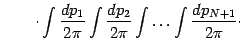
Next, one has to determine an equation for the partial amplitude
(5)
that the system evolves from a position with coordinate
at time to a position with coordinate
at time .
Using the bracket notation, the amplitude for the first
subinterval takes the form
(6)
Generalizing the above expression to a generic subinterval, we find
(7)
Approximating the path from at time to at time
with a finer subdivision of the total time interval,
and in view of the fact that there are no predetermined
conditions on the coordinate variable at intermediate times,
the total amplitude can be written as the product
of the amplitudes associated with each subinterval, integrated
over all possible intermediate positions:
(8)
Combining the two equations above, we are led to the
final step of the discretization procedure
The expression in the last equality represents
the discrete version of the path integral in phase space
(9)
which is the starting point for computing
the sum over histories for the majority of
the integrable systems encountered in the
literature. Equation (9)
is also the starting point of our own approach.
However, in terms of the discretization procedure
outlined above, a further simple elaboration of
the phase space path integral leads to a computational
method which seems mathematically more efficient and
physically more enlightening, at least for some complex
systems encountered in high energy physics.
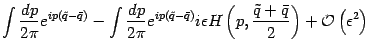
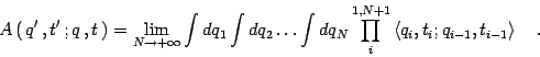
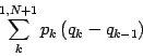
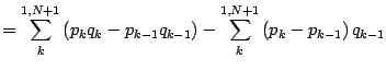
Consider the first term in the expression (9), namely
(10)
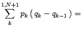
This term corresponds to the discrete sum
(11)
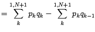
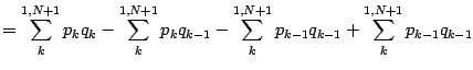
which we can rewrite as follows:
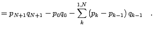
(12)
The first two terms in the above expression represent a boundary
contribution to the path integral, whereas the
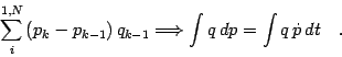
remaining sum corresponds to the following integral
(13)
Next, in what follows we make use of the following equality
(14)
which gives the well known representation of the Dirac delta function as
Fourier transform of the imaginary exponential.
Thus, the net result of the above rearrangement
of terms is encoded in the following correspondence
(15)
which we take as a definition of the
``functional Dirac delta distribution''.
In the next section, we apply this mathematical
rearrangement of terms in the phase space path
integral to compute the propagation kernel of a
non relativistic particle. As we shall see, the
physical payoff is a novel interpretation of the
sum over histories in the sense that it underscores
the special role played by the entire family of
trajectories which are solutions of the classical
equations of motion.
![$\displaystyle \int \frac{dp}{2 \pi}
e ^{i p \left( \tilde{q} - \bar{q} \right)}...
...{q} + \bar{q}}{2} \right)
\right ]
+ {\mathcal{O}} \left( \epsilon ^{2} \right)$](img31.gif)
![$\displaystyle \int \frac{dp}{2 \pi}
\exp
\left\{
i
\left [
p \left( \tilde{q} -...
...on
H \left( p , \frac{\tilde{q} + \bar{q}}{2} \right)
\right ]
\right\}
\quad .$](img32.gif)
![$\displaystyle \qquad \qquad \qquad \qquad \cdot
e ^{i \left [
p _{N+1} \left(...
...\right)
H \left( p _{N+1} , \frac{q _{N+1} + q _{N}}{2} \right)
\right]
}$](img44.gif)
![$\displaystyle \qquad \cdot
e ^{i \left \{
\sum _{k} ^{1,N+1}
\left[
p _{k} \lef...
...ight)
H \left( p _{k} , \frac{q _{k} + q _{k-1}}{2} \right)
\right ]
\right\}
}$](img46.gif)
![$\displaystyle \qquad \cdot
e ^{i \left \{
\sum _{k} ^{1,N+1}
\left[
p _{k} \fra...
..._{k-1}}{2} \right)
\right ]
\left( t _{k} - t _{k-1} \right)
\right\}
}
\quad .$](img47.gif)
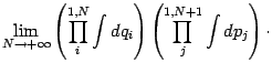
![\begin{displaymath}
\int \left [ {\mathcal{D}} q \right]
\exp \left\{ i \int d...
... \frac{p _{k} - p _{k-1}}{t _{k} - t _{k-1}}
\right)
\quad .
\end{displaymath}](img58.gif)