In this subsection, as already anticipated above, we wish to discuss
in more detail the case of open ![]() -branes endowed with electric charge
only, in order to emphasize in a simpler case the peculiarities of the
open case with respect to the closed one that we have summarized in
section 2. In particular it is important to observe the
physical (extended!) origin of the field content in the action of the
starting theory. Honoring the procedure we employed so far, we associate
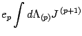
to each extended object a source current, coupled to a suitable gauge
potential, which in turn ``generates'' a field strength in the
-branes endowed with electric charge
only, in order to emphasize in a simpler case the peculiarities of the
open case with respect to the closed one that we have summarized in
section 2. In particular it is important to observe the
physical (extended!) origin of the field content in the action of the
starting theory. Honoring the procedure we employed so far, we associate
to each extended object a source current, coupled to a suitable gauge
potential, which in turn ``generates'' a field strength in the
![]() -dimensional spacetime. The source current is divergenceless, i.e.
the corresponding charge is conserved, only if the associated object is
closed; moreover under this condition the theory is gauge invariant,
since ``going to the boundary'' in the action integral yields no
``breaking terms'': indeed for closed objects there is no boundary at
all. After this remarks it is thus clear the way in which the open case
differs from the closed one. The source current of the open
-dimensional spacetime. The source current is divergenceless, i.e.
the corresponding charge is conserved, only if the associated object is
closed; moreover under this condition the theory is gauge invariant,
since ``going to the boundary'' in the action integral yields no
``breaking terms'': indeed for closed objects there is no boundary at
all. After this remarks it is thus clear the way in which the open case
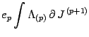
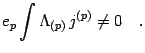
differs from the closed one. The source current of the open ![]() -brane is
not divergenceless now, due to the presence of the boundary (which is
a
-brane is
not divergenceless now, due to the presence of the boundary (which is
a ![]() -brane). Hence there is a leakage of current through the boundary,
and this breaks the gauge symmetry of the action
-brane). Hence there is a leakage of current through the boundary,
and this breaks the gauge symmetry of the action
 |
|||
 |
|||
 |
(32) |
Thus the gauge invariant form of the closed action (31)
in the open case is
Now we will see how, the presence of a boundary, and thus of a
further interaction on it mediated by the Stückelberg field, can be
traded off with a massive interaction within the ![]() -brane elements:
in some sense, we can forget about the presence of the boundary, when
we concentrate on the gauge invariance properties of the theory, and
simply reinterpret it as the propagation of massive degrees of freedom
on the
-brane elements:
in some sense, we can forget about the presence of the boundary, when
we concentrate on the gauge invariance properties of the theory, and
simply reinterpret it as the propagation of massive degrees of freedom
on the ![]() -dimensional extended object. This is seen as follows.
-dimensional extended object. This is seen as follows.
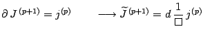
First, we derive from the action (33) the field equations,
by means of variations with respect to the two gauge potentials, ![]() and
and ![]() , respectively:
, respectively:
|
|
(38) |
|
|
(39) |
 |
(40) |
|
|
(41) |
|
|
(42) |
 |
(43) |
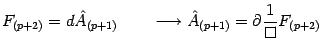
Then, we get from eq.(37)
 |
(44) |
while, the Maxwell-like (36) equation can be written in terms of the field strength as
| (45) |
Third, we substitute the solutions into the action (33)
and we get,
As a consequence of the gauge invariance (35) introduced by the
Stückelberg conpensator the action (46) is written in terms
of divergence free currents. The first term in (46) represents a
short range, bulk interaction mediated by a massive vector
boson, as it could be expected since the very beginning. However, this is
conclusion less trivial than it could appear at first sight: we have no
Higgs Model for ![]() -branes and no way to break gauge symmetry spontaneously.
At present, the only, gauge invariant way to provide a mass
tensor gauge field with a mass term is through the Stückelberg mechanism
discussed above. The cosmological implications of this new conversion
mechanism, transforming the vacuum energy ``stored'' by a massless
tensor gauge potential into massive particles is currently under
investigation[12].
-branes and no way to break gauge symmetry spontaneously.
At present, the only, gauge invariant way to provide a mass
tensor gauge field with a mass term is through the Stückelberg mechanism
discussed above. The cosmological implications of this new conversion
mechanism, transforming the vacuum energy ``stored'' by a massless
tensor gauge potential into massive particles is currently under
investigation[12].
Finally, the last term in (46) describe a long range
interaction confined on the boundary. With hindsight we can
recognize this term as the memory of the interaction mediated
by the massless Stückelberg field ![]() . In a sort of Meissner-like
effect the conpensator is `` expelled '' form the bulk and trapped over
the boundary of the extended object. It has been suggested that
in the limiting case
. In a sort of Meissner-like
effect the conpensator is `` expelled '' form the bulk and trapped over
the boundary of the extended object. It has been suggested that
in the limiting case ![]() this ``secret long range force'' can produce
confinement, in
this ``secret long range force'' can produce
confinement, in ![]() , and glueball formation in
, and glueball formation in ![]() [13].
Accordingly, we expect similar effects in higher dimensions [6].
[13].
Accordingly, we expect similar effects in higher dimensions [6].
The above effects represent the physical output of the Stückelberg
Mechanism for electric ![]() -branes. To investigate the strong coupling
dynamics of this mechanism we have to switch to the `` magnetic phase ''
of the model (31). The condition (7) guarantees that
a strong electric coupling regime can be equivalently described in terms
of a dual weak magnetic coupling phase.
Thus, duality procedure can now be developed, but we defer it to the next
subsection, since the same set-up can be now applied in the more general case
in which electric as well as magnetic charges are present.
-branes. To investigate the strong coupling
dynamics of this mechanism we have to switch to the `` magnetic phase ''
of the model (31). The condition (7) guarantees that
a strong electric coupling regime can be equivalently described in terms
of a dual weak magnetic coupling phase.
Thus, duality procedure can now be developed, but we defer it to the next
subsection, since the same set-up can be now applied in the more general case
in which electric as well as magnetic charges are present.
![$\displaystyle {1 \over Z [ \, 0 \, ]}
\int [ {\mathcal{D}}A ] [ {\mathcal{D}}C ]
\,
e ^{ - S [ \, A , C , J _{\mathrm{e}} \, ]}$](img119.gif)
![$\displaystyle \int
\left [ - { 1\over 2 } F _{(p+2)} F ^{\, (p+2)} - { \kappa\o...
... (p+2)} - e _{p} \,
F _{(p+2)}\, d{ 1 \over \Box }\hat{J}^{\, (p+1)}\,
\right ]$](img141.gif)
![$\displaystyle \int
\left [\, -{ e _{p}^2\over 2 }
\hat{J} ^{\, (p+1)}
\frac{1}{...
...
+ { e _{p}^2 \over 2\kappa }
j ^{(p)}
\frac{1}{\Box}
j ^{(p)}
\right ]
\quad .$](img142.gif)